Edwards on Fisher (2005)

In his discussion of Fisher's 1925 book Statistical Methods for Research Workers, Edwards writes:

It was not until 1950 that the word ‘Bayesian’ was coined, by Fisher himself, to refer to inverse probability (p. 862)

Can this really be true? To be sure, "inverse probability" was the more common term before 1950, but was "Bayesian" really never used, at all?

I thought this claim would not stand up to 30 seconds of googling, but I was wrong. The only reference I've found so far is from the bibliography in Jimmy Savage's Lecture Notes on Mathematical Statistics, which includes the following item:

Jeffreys, Harold. Theory of Probability. New York: Oxford University Press, 1939. 380 pp. A highly controversial book on the philosophical foundations of statistics by the most foremost modern exponent of the Bayesian heresy. Examples largely from geophysics.

I don't have access to Savage's book here, so I can't vouch for the year of publication, but Amazon, WorldCat, Google Books, and a few other resources all give the date as 1947.

If that's true, then the word "Bayesian" was used at least once before 1950. But one is certainly not a crowd.

Chrystal: "On Some Fundamental Principles in the Theory of Probability" (1891)

I've been trying to get my hands on the following paper:

George Chrystal (University of Edinburgh): "On Some Fundamental Principles in the Theory of Probability." Transactions of the Actuarial Society of Edinburgh, Volume 2, January 1891, pages 420–439.

So far, no luck. The Cambridge Journals database has a copy, but it's behind a paywall, and my university doesn't have a subscription.

However, a number of other sources quote extensively from the paper, so I've been able to piece together an understanding of what it looks like.

Posterior Frequencies

It seems that Chrystal's main beef is with the use of Bayes' rule to update the probability of a certain set of hypotheses whose long-term frequencies are already given in advance. His reasoning seems to be that this conflates our subjective degree of belief (which may indeed change) with the objective frequency (which, by assumption, cannot).

This philosophical distinction is nicely presented in the following quote. It comes from an 1894 review (also available in book form on the Internet Archive) by somebody called G. F. Hardy, not to be confused with G. H. Hardy.

"There is," says Professor Chrystal, "in Laplace's view, a confusion between two senses of the word 'Probability', which although distinct are often more or less associated in point of fact. In common speech we say that a single event is more or less 'probable', and by this word we indicate our own mental attitude towards the event, an attitude that may be well or ill justified by facts. When an actuary says that the probability that a man of 20 will live to be 60 is $\frac{59}{97}$, he is not, strictly speaking, referring to any one event at all, but merely making an assertion to the effect that out of any considerable number of men of 20 years of age about $\frac{59}{97}$ will reach the age of 60. No one knows better than an actuary that this statement is a fact, established (under certain circumstances, and with certain limitations), by experience, and that it has nothing whatever to do with the mental attitude of anyone. Everyone will admit that we could never arrive at this result by analyzing the event of a man of 20 reaching or not reaching the age of 60 into cases regarding each of which we should be equally undecided,—mentally suspended, as it were, like Buridan's ass between the equal bundles of hay." (Hardy, p. 316)

It's not clear whether the emphases are in the original, but I'm guessing not.

Hardy does not give a page reference, but proper reference seems to be page 423. I got that figure from the manuscript of a 1893 presentation by a certain John Govan, F.F.A. (whose name, location, and date fit the proselytizing businessman John George Govan).

Govan's rendition of the quote occurs on his page 212. He doesn't use the emphases.

The Burial of Bayes

Several sources also report that Chrystal summarizes his discussion with the following tirade:

… both from the point of view of practical common-sense, and from the point of view of logic, the so-called laws of Inverse Probability are a useless appendage to the first principles of probability, if indeed they be not a flat contradiction of those very principles.

This is cited by a number of authors, including E. T. Whittaker, F.R.S. (in a footnote to a 1920 presentation, p. 165), Andrew I. Dale (1999, p. 485) and Sharon McGrayne (2011, p. 37).

Dale reports that this quote is found on page 438. Whittaker apparently reports it as page 421 (but that would be at odds with Dale's description of the quote as a occurring near the conclusion of the essay). McGrayne doesn't give a page number.

According to Whitaker, the quote continues as follows:

The laws of Inverse Probability being dead, should be decently buried out of sight, and not embalmed in text-books and examination papers.

McGrayne further reports the following conclusion:

The indiscretions of great men should be quietly allowed to be forgotten.

Checking the relevant footnote of McGrayne's book (note 9 of ch. 3, p. 260), this turns out to be a recycled quote from Anders Hald's A History of Mathematical Statistics, page 275. That book doesn't have a Google Books preview, and it's not in my library.

Sort-of-Long-Term Frequencies

Hardy's review continues to quote Chrystal's discussion of how probability is to be defined:

"The notion of probability is always attached to a class or series of events, which usually have more or less of other attributes in common, but are always distinguished by this mark, that certain phases of them, although not predicable with the smallest certainty in any individual case, are predicable with more or less uniformity in a certain proportion of cases in the long run. The fundamental features of this series are statistical uniformity combined with irregularity of every conceivable kind in the individual instance. The number of the events in the series must be large. Its extension both as to space and time is arbitrary, and in certain ideal cases infinite. It is in this last respect alone that probability has anything to do with our mental attitude; we may choose our standpoint, and this determines the probability to which our knowledge may make a better or worse approximation. As the series is varied the probability alters. . . .  We are thus led to the following abstract definition of the probability or chance or an event. If, on taking any very large number, N out of a series of cases in which an event A is in question, A happens on pN occasions, the probability of the event A is said to be p." (Hardy, p. 317)

Again, no page number is given.

Posterior Priors

The examples in Chrystal's paper seem all to be of the same kind: He describes a set-up in which certain a priori frequencies are given, and he then tells us that no amount of evidence should be able to change those frequencies; the only mental operation we can perform is to exclude logically impossible cases, not to compute posterior probabilities.

Govan thus quotes him as discussing a situation in which you draw two white balls from a bag of black and white balls. Then:

"Any one," says Professor Chrystal, "who knows the definition of mathematical probability, and who considers this question apart from the Inverse Rule, will not hesitate for a moment to say that the chance is $\frac{1}{2}$; that is to say, that the third ball is just as likely to be white as black. For there are four possible constitutions of the bag . . . each of which we are told occurs equally often in the long run, and among those cases there are two . . . in which there are two white balls, and among these the case in which there are three white occurs in the long run, just as often as the case in which there are only two." (Govan, p. 208)

According to the text of Govan's discussion, this quote must be on or around page 435 of Chrystal's text.

Another very similar example is attributed to Chrystal's page 437:

"A bag contains five balls which are known to be either all black or all white—and both these are equally probable. A white ball is dropped into the bag, and then a ball is drawn out at random and found to be white. What is now the chance that the original balls were all white?" Professor Chrystal asserts that the chance is precisely what it was before, viz. $\frac{1}{2}$. (Govan, p. 208–209)

"The ball drawn out," says Professor Chrystal, "may have been the one we put in, it may not; and this is all that any one can say." (Govan, p. 209)

Note that this is quite upside-down compared to how we usually think about frequentism: Here, Chrystal tells us to ignore the likelihoods and put all our confidence in the priors. We are used to thinking about frequentists as doing the exact opposite.

The Essential Tension

Govan objects to Chrystal's principle of rejecting the evidence:

… let us say we have two bags before us, one containing six white balls, the other five black balls and one white. There is nothing to indicate which is which. We draw from one of the bags chosen at random a ball which proves to be white. It is difficult to believe that any man in the possession of his faculties, say if his life depended on his guessing aright from which bag the ball had come, would hesitate to guess the former. Even according to Professor Chrystal he would be right 6 times out of 7 in the long run. Yet, again according to Professor Chrystal he would would be just as likely to be wrong as to be right. (Govan, p. 209)

Although they are talking past each other, this is certainly the core of the issue: The distinction between optimal, adaptive gambling behavior and fixed, objective frequencies.

Edwards: Likelihood (1972)

Edwards (from his Cambridge site)

The geneticist A. F. W. Edwards is a (now retired) professor of biometry who was massively influenced by Ronald Fisher in his scientific writings. His books Likelihood argues that the likelihood concept is the only sound basis for scientific inference, but it reads at times almost like one long rant against Bayesian statistics (particularly ch. 4) and Neyman-Pearson theory (particularly ch. 9).

Don't Do Probs

As an alternative to these approaches to statistics, Edwards proposes that we limit ourselves to makes assertions only in terms of likelihood, "support" (log-likelihood, p.12), and likelihood ratios. In the brief epilogue of the book, he states that this

… allows us to do most of the things which we want to do, whilst restraining us from doing some things which, perhaps, we should not do. (p. 212)

In particular, this approach emphatically prohibits the comparison of hypotheses in probabilitistic terms. The kind of uncertainty we have about scientific theories is simply not, Edwards states, of a nature that can be quantified in terms of probabilities: "The beliefs are of a different kind," and they are "not commensurate" (p. 53)

The Difference Between Bad and Worse

He briefly mentions Ramsey and his Dutch book-style argument for the calculus of probability, and then goes on to speculate that, had not died so young,

… perhaps he would have argued that his demonstration that absolute degrees of belief in propositions must, for consistency's sake, obey the law of probability, did not compel anyone to apply such a theory to scientific hypotheses. Should they decline to do so (as I do), then they might consider a theory of relative degrees of belief, such as likelihood supplies. (p. 28)

In other words, it might be true that you cannot assign numbers to propositions in any other way than according to the calculus of probabilities, but you can always reject to have a quantitative opinion in the first place (or not make a bet).

Nulls Only

Consistently with Fisher's approach to statistics, Edwards finds it important to distinguish between null and not-null hypotheses: That is, in opposition to Neyman-Pearson theory, he refuses to explicitly formulate the alternative hypothesis against which a chance hypothesis is tested.

Here as elsewhere, this is a serious limitation with quite profound consequences:

It should be noted that the class of hypotheses we call 'statistical' is not necessarily closed with respect to the logical operations of alternation ('or') and negation ('not'). For a hypothesis resulting from either of these operations is likely to be composite, and composite hypotheses do not have well-defined statistical consequences, because the probabilities of occurrence of the component simple hypotheses are undefined. For example, if $p$ is the parameter of a binomial model, about which inferences are to be made from some particular binomial results, '$p=\frac{1}{2}$' is a statistical hypothesis because its consequences are well-defined in probability terms, but its negation, '$p\neq\frac{1}{2}$', is not a statistical hypothesis, its consequences being ill-defined. Similarly, '$p=\frac{1}{4}$ or $p=\frac{1}{2}$' is not a statistical hypothesis, except in the trivial case of each simple hypothesis having identical consequences. (p. 5)

This should also be contrasted with Jeffreys' approach, in which the alternative hypothesis has a free parameter and thus is allowed to 'learn', while the null has the parameter fixed at a certain value.

Scientists With Attitude

At several points, in the book, Edwards uses the concerns of the working scientist as an argument in favor of a likelihood-based reasoning calculus. He thus faults Bayesian statistics for "fail[ing] to answer questions of the type many scientists ask" (p. 54).

This question, I presume, is "What does the data tell my about my hypotheses?" This is distinct from "What should I do?" or "Which of these hypotheses is correct?" in that it only supplies the objective, quantitative measure of support, not the conclusion:

The scientist must be the judge of his own hypotheses, not the statistician. The perpetual sniping which statisticians suffer at the hands of practising scientists is largely due to their collective arrogance in presuming to direct the scientists in his consideration of hypotheses; the best contribution they can make is to provide some measure of 'support', and the failure of all but a few to admit the weaknesses of the conventional approaches has not improved the scientists' opinion. (p. 34)

In brief form, this leads to the following tirade against Bayesian statistics:

Inverse probability, in its various forms, is considered and rejected on the grounds of logic (concerning the representation of ignorance), utility (it does not allow answers in the form desired), oversimplicity (in problems involving the treatment of frequency probabilities) and inconsistency (in the allocation of prior probability distributions). (p. 67–68)

Fisher: The Design of Experiments (4th ed., 1947), Chapter I

Fisher; from Judea Pearl's website.

Now, here's a revealing turn of phrase:

In the foregoing paragraphs the subject-matter of this book has been regarded from the point of view of an experimenter, who wishes to carry out his work competently, and having done so wishes to safeguard his results, so far as they are validly established, from ignorant criticism by different sorts of superior persons. (p. 3)

You could hardly spell out more explicitly the philosophy that lies behind Fisher's concept of statistics: It's a strategic ritual, not designed to ensure a result, but to protect against criticism.

Perfectly Rigorous and Unequivocal

Such protection only goes as far as the mathematical consensus on the validity of the logic. But Fisher goes on to state that "rigorous deductive argument" is possible even in the context of random events, citing gambling as a proof of concept:

The mere fact that inductive inferences are uncertain cannot, therefore, by accepted as precluding perfectly rigorous and unequivocal inference. (p. 4)

This seems to confuse the issues of probability and statistics, unless his argument here really only amounts to saying that distributions are non-stochastic entities.

Useless for Scientific Purposes

This leads him to a discussion of "inverse probability," which he gives three reasons for rejecting: First,

… advocates of inverse probability seem forced to regard mathematical probability, not as an objective quantity measured by observed frequencies, but as measuring merely psychological tendencies, theorems respecting which are useless for scientific purposes. (p. 6–7)

Second, Bayes' axiom (about the flat prior for a coin flip) is not self-evident, that is, the choice of prior is not unequivocal (p. 7).

Ever Since the Dawn of Man…

And third,

… inverse probability has been only very rarely used in the justification of conclusions from experimental facts, although the theory has been widely taught, and is widespread in the literature of probability. Whatever the reasons are which could give experimenters confidence that they can draw valid conclusions from their results, they seem to act just as powerfully whether the experimenter has heard of the theory of inverse probability or not. (p. 7)

That's a funny sociological proof, given that he has just rejected Bayesian statistics for its psychologism. But he himself sometimes seems to think that his statistics is a kind of theory of learning, whatever that means:

Men have always been capable of some mental processes of the kind we call "learning by experience." … Experimental observations are only experience carefully planned in advance, and designed to form a secure basis of new knowledge; (p. 8)

Chernoff: "A career in statistics" (2014)

Chernoff makes some interesting remarks about the philosophy of statistics in his recent autobiographical essay.

First, an anecdote about the three classical decision criteria considered in decision theory:

I had always been interested in the philosophical issues in statistics, and Jimmie Savage claimed to have resolved one. Wald had proposed the minimax criterion for deciding how to select one among the many “admissible” strategies. Some students at Columbia had wondered why Wald was so tentative in proposing this criterion. The criterion made a good deal of sense in dealing with two-person zero-sum games, but the rationalization seemed weak for games against nature. In fact, a naive use of this criterion would suggest suicide if there was a possibility of a horrible death otherwise. Savage pointed out that in all the examples Wald used, his loss was not an absolute loss, but a regret for not doing the best possible under the actual state of nature. He proposed that minimax regret would resolve the problem. At first I bought his claim, but later discovered a simple example where minimax regret had a similar problem to that of minimax expected loss. For another example the criterion led to selecting the strategy A, but if B was forbidden, it led to C and not A. This was one of the characteristics forbidden in Arrow’s thesis.

Savage tried to defend his method, but soon gave in with the remark that perhaps we should examine the work of de Finetti on the Bayesian approach to inference. He later became a sort of high priest in the ensuing controversy between the Bayesians and the misnamed frequentists. (pp. 32–33)

He immediately moves on to one of his own more dismal conclusions about the issue:

I posed a list of properties that an objective scientist should require of a criterion for decision theory problems. There was no criterion satisfying that list in a problem with a finite number of states of nature, unless we canceled one of the requirements. In that case the only criterion was one of all states being equally likely. To me that meant that there could be no objective way of doing science. I held back publishing those results for a few years hoping that time would resolve the issue (Chernoff, 1954). (p. 33)

I haven't read the paper he is referring to here, but it seems like the text has jumbled up the conclusions: I think what he meant to say is that there is no single good decision function when we have infinitely many states, since the criteria essentially require us to use a uniform distribution. But I would have to check the details.

Finally, he moves on to a more on-record explication of his position:

In the controversy, I remained a frequentist. My main objection to Bayesian philosophy and practice was based on the choice of the prior probability. In principle, it should come from the initial belief. Does that come from birth? If we use instead a non-informative prior, the choice of one may carry hidden assumptions in complicated problems. Besides, the necessary calculation was very forbidding at that time. The fact that randomized strategies are not needed for Bayes procedures is disconcerting, considering the important role of random sampling. On the other hand, frequentist criteria lead to the contradiction of the reasonable criteria of rationality demanded by the derivation of Bayesian theory, and thus statisticians have to be very careful about the use of frequentist methods. 

In recent years, my reasoning has been that one does not understand a problem unless it can be stated in terms of a Bayesian decision problem. If one does not understand the problem, the attempts to solve it are like shooting in the dark. If one understands the problem, it is not necessary to attack it using Bayesian analysis. My thoughts on inference have not grown much since then in spite of my initial attraction to statistics that came from the philosophical impact of Neyman–Pearson and decision theory. (p. 33)

Duda and Hart: Pattern Classification and Scene Analysis (1973)

A lot of references seem to indicate that this book played an important role in the popularization of Bayesian methods in machine learning. It also provides an interesting missing link between the statistics and decision theory of the 1950s and the field of machine learning in the form it now has.

Interestingly, their rejection of minimax approaches to decision theory is rather casual, relative to how toxic the debate actually was:

In fact, the Bayesian approach is avoided by many statisticians, partly because there are problems for which a decision is made only once (so that average loss is not meaningful), and partly because there may be no reasonable way to determine the a priori probabilities. Neither of these difficulties seems to present a serious problem in typical pattern recognition applications, and for simplicity we have taken a strictly Bayesian approach. (p. 36)

Compare this to David Blackwell's compact statement of intent in Basic Statistics (1969):

This book indicates the content of a lower-division basic statistics course I have taught several times at Berkeley. […] The approach is intuitive, informal, concrete, decision-theoretic, and Bayesian. (p. v)

Duda and Hart also provide a number of quite interesting references:

The text by Nilsson (1965) provides an exceptionally clear treatment of classification procedures. (p. 8)

There are many interesting subject areas that are related to this book but beyond its scope. […] Those interested in philosophical issues will find the books by Watanabe (1969) and Bongard (1970) thought provoking. (p. 8)

We are also fond of the the text by Ferguson (1967), who presents many topics in statistics from a decision theoretic viewpoint. (p. 36)

Chow (1957) was one of the first to apply Bayesian decision theory to pattern recognition. His analysis include a provision for rejection, and he later estiablished a funcamental relation between error and reject rates (Chow 1970). (p. 36)

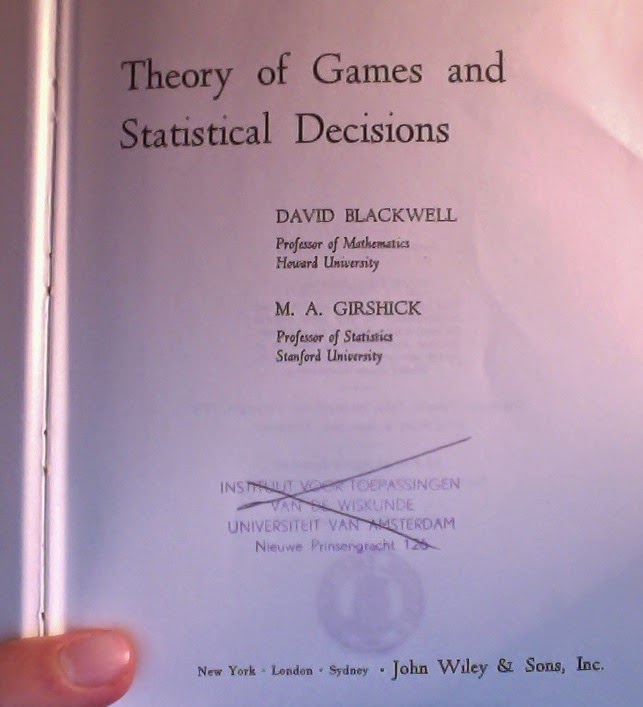
Blackwell and Girshick: Theory of Games and Statistical Decisions (1954), Ch. 4

There's an interesting representation theorem in Blackwell and Girshick's textbook in statistics: It provides a set of sufficient conditions for a preference ordering over lotteries to be expressible as a prior probability distribution (Th. 4.3.1, p. 118).

I assume the theorem comes from either Wald, Savage, or de Finetti, but no reference is given.

Well-Behaved Preferences

A lottery can here be defined as a function from the sample space to the real numbers. The conditions in the theorem are then the following:

• The ordering of two lotteries $f$ and $g$ cannot depend on the availability of other lotteries.
• If a lottery $f$ provides a higher payoff than a lottery $g$ at all points in the sample space $\Omega$, then $f$ must be preferred to $g$.
• If $f$ is preferred to $g$, then $f+h$ must be preferred to $g+h$.

An inspection of the proof also shows that they should have included a continuity condition:

• If $f_1, f_2, \ldots$ is a series of lotteries converging to a limit $f$, and if $f_i$ is preferred to $g$ for all $i$, then $f$ must also be preferred to $g$.

When these conditions are met, the preference ordering over the lotteries can be expressed as a distribution over the sample space, unless it categorizes all lotteries as equally good.

The Large and the Good

The proof of the theorem uses the fact that two convex, disjoint, open sets can be separated by a hyperplane. Here's a sketch:

If we let $e$ be the lottery that pays zero in all situations $\omega \in \Omega,$ then we can define the following sets:
\begin{eqnarray}
F[>] &=& \{f\ |\ \forall \omega \in \Omega: f(\omega) > 0\},
\\
F[\gtrsim] &=& \{f\ |\ f\gtrsim e\},
\end{eqnarray}
and we can further define, in the usual way, $F[>] + F[\gtrsim]$ to be the sums of lotteries from those two sets.

Now, $F[>]$ is an open set, and hence $F[>] + F[\gtrsim]$ is, too. Further, $F[>]$ and $F[\gtrsim]$ are both closed under addition (due to the third assumption), and hence their sum is, too. They are also both closed under multiplication with a scalar, and again, so is their sum — but this latter argument requires a bit more spelling out.

Rational and Real Convexity

Suppose a lottery $f$ is preferred to the zero lottery, that is, $f \in F[\gtrsim]$. The third assumption of the theorem then tells us that
$$
e \;\lesssim\; f \;\lesssim\; f + f \;\lesssim\; f + f + f \;\lesssim\; \ldots \;\lesssim\; nf.
$$
By further adding multiple copies of the zero lottery to both sides of this preference ineqality, we can see that
$$
me \;\lesssim\; (m-1)e + nf \;=\; nf,
$$
where we have selectively used the fact that $e$ is the zero lottery. Putting these facts together, we then have the preference inequality
$$
e \;\lesssim\; \left(\frac{n}{m}\right)f.
$$
By using a positive sequence of rational approximations $(n/m) \rightarrow \lambda$, we can use this fact along with the continuity assumption to conclude that $F[\gtrsim]$ is closed under multiplication with any positive, real scalar $\lambda$.

I don't think there's a way around this last technicality. It is, incidentally, the same proof technique used to prove that the logarithmic functions are the only continuous functions that turn products into sums.

Cutting the Cake

At any rate, $F[>] + F[\gtrsim]$ is an open and convex set separated from the singleton set $\{e\}$. We can therefore conclude that there is a lottery (or vector) $p$ which defines the hyperplane $\{f\ |\ f\cdot p=0\}$ separating $F[>] + F[\gtrsim]$ from $\{e\}$. The set $F[>] + F[\gtrsim]$ is thus a subset of the half-space $\{f\ |\ f\cdot p \geq 0\}$.

This vector $p$ must have nonnegative coordinates, since the set $F[>]$ is unbounded in all positive directions. If $p$ had a negative coordinate, $p(\omega) \leq 0$, we could choose a lottery for which the corresponding coordinate, $f(\omega)$, was so large that $f\cdot p < 0$. This would violate the definition of $p$, and $p$ hence has to be a nonnegative vector which can be interpreted as a probability distribution.

It would also have the property that $f\cdot p \geq g\cdot p$ if and only if $f \gtrsim g$. This follows from the fact that $f\cdot p \geq g\cdot p$ if and only if $(f - g) \in F[>] + F[\gtrsim]$, which holds if and only if $f$ can be expressed as the sum of $g$ and some lottery preferable to the zero lottery.

Baker, Saxe, and Tenebaum: "Bayesian Theory of Mind" (2011)

I was referred to this paper by one of the reviewers of my own paper on multi-agent statistics, since both seemed to be about reasoning about other people's beliefs. Their paper is concerned with inferring one other person's belief-desire state from observed behavior, not with reasoning of arbitrarily high order (like I know that you know that I know…). This means that there are some issues in general multi-agent statistics that they don't have to worry about.

At any rate, the set-up they consider is the following:

• The subject observes a little stylized scene comparable to a simple video game interface.
• This scene features a little cartoonish character (a circle with two eyes).
• Depending on where the character is standing, different parts of the scene will be blocked from view.
• The scene contains two parking lots in which food trucks can park.
• There are three different kinds of food truck that may or may not be present in the scene.
• In each condition, the subject sees the little character move around in a certain predetermined way.

After watching this scene, the subjects were then asked to provide assessments of the little character's beliefs and food preferences. For instance, if the character could initially see a truck with Korean food, but still walked up to check the other parking lot, this must be because the person was wondering whether a more preferred kind of food was available.

The character sees the Korean truck, yet walks up and checks what else is available.

In the model, these videos were discretized and treated as a hidden Markov model with the desires (food preference ordering) and beliefs (about which trucks there might be in the parking lots) as hidden states.

At each time step, previous actions inform new states of the world.

Since there were actually a quite small space of possible routes and possible plans, the model could in fact have been simplified immensely in this case, although at the expense of generalizability.

Wald: Sequential Analysis (1947)

I've always thought that Shannon's insights in the 1940s papers seemed like pure magic, but this book suggests that at parts of his way of thinking were already in the air at the time: From his own frequentist perspective, Wald comes oddly close to defining a version of information theory.

The central question of the book is:

How can we devise decision procedures that map observations into {Accept, Reject, Continue} in such a way that (1) the probability of wrongly choosing Accept or Reject is low, and (2) the expected number of Continue decisions is low?

Throughout the book, the answer that he proposes is to use likelihood ratio tests. This puts him strangely close to the Bayesian tradition, including for instance Chapter 5 of Jeffreys' Theory of Probability.

A sequential binomial test ending in rejection (p. 94)

In particular, the coin flipping example that Jeffreys considers in his Chapter 5.1 is very close in spirit to the sequential binomial test that Wald considers in Chapter 5 of Sequential Analysis. However, some differences are:

• Wald compares two given parameter values p₀ and p₁, while Jeffreys compares a model with a free parameter to one with a fixed value for that parameter.
• Jeffreys assigns prior probabilities to everything; but Wald only uses the likelihoods given the two parameters. From his perspective, the statistical test will thus have different characteristics depending on what the underlying situation is, and he performs no averaging over these values.

This last point also means that Wald is barred from actually inventing the notion of mutual information, although he comes very close. Since he cannot take a single average over the log-likelihood ratio, he cannot compute any single statistic, but always has to bet on two horses simultanously.

Wolpert: "The Lack of A Priori Distinctions Between Learning Algorithms" (1996)

I think this might be one of the most oversold math papers I've ever read. The core idea of the paper is a tiny little nugget of common sense buried under a mountain of notation. This not only makes the paper hard to read, but also camouflages the heavy-handed assumptions that are necessary to make the argument work.

No Lunch At All

The learning scenario that Wolpert studies in the paper is one in which we want to guess the values of a function f: X → Y when evaluated on input values that did not occur in our training data. We do so by selecting an estimate h: X → Y, hoping that h(x) will agree with f(x) on the points x we haven't yet seen.

If there no restrictions on how f can be chosen, and all of the exponentially many underlying functions are possible, then no such generalization is possible. Whatever h we choose, Wolpert can always choose f so as to disagree with every single choice that our h makes outside the training set, or (if he should so desire) so as to agree with all of them.

In other words, if everything is possible, then there is no statistical dependency between the past and the future. Obviously, this means that learning is impossible.

Extremely Large and Incredibly Bold

Let me just elaborate this last reformation a bit more:

Suppose your data consists of a binary sequence of length m, and your goal is to predict the next n binary digits in the sequence. If all of the 2^{n + m} possible sequences are in your hypothesis space, then the mutual information between the test and training set is

I(train; test)  =  H(test)  –  H(test | train)  =  2ⁿ  –  2^n + m/2^m  =  0.

In such a case, you might as well guess randomly. However, this only follows because the set of possible sequences has an entropy rate of 1, and because you only care about exactly correct guesses (otherwise the sequence 1/2, 1/2, 1/2, … might outperform random 0/1 guessing).

If It's Independent, It's Independent

To say this in a more Wolpert way, let's make the following definitions:

• A loss measure L is "homogenous" if our choice of the estimate h is independent of the sum of the loss probabilities given the correct answers, that is,

  Σ_y Pr{L = c | y}.

• For finite |X| and |Y|, we can define a learning problem as uniform if all of the |Y|^|X| possible functions from X to Y are equally probable.
• When we use a homogenous loss function in a uniform learning problem, then

  Σ_y Pr{L = c | y}  =  1/|Y| Σ_y Pr{L = c | y} Pr{y}  =  1/|Y| Pr{L = c}

  is independent of h, and therefore E[L | h] = E[L].

Combining homogeneity and uniformity is thus the same as assuming that the loss is independent of the learning algorithm.

The Don't-Get-Cute Condition

The zero-one loss function (which gives you one point for each correct answer) is "homogenous" in this sense, but it is pretty much the only one. For most other loss functions, it will often make sense to use some central value as your guess for f(x), since extreme guesses are panelized more heavily under a uniform selection scheme.

As an example, consider the loss function L(f(x), h(x)) = |f(x) – h(x)|, and suppose we are trying to guess an unknown number in the set {1, 2, 3, 4, 5}. Then the probability that L = 4, for instance, depends heavily on your estimator h, since an estimate that never returns the values 1 or 5 can never achieve this loss. Numerical deviation is therefore not "homogenous," and neither is ordinary squared deviations.

The Maximally Expensive Lunch

Naturally, Wolpert wants to discuss the relation between his own paper and the uniform law of large numbers, proven by Vapnik and Chervonenkis in the late '60s.

He thus states that if we are using a homogenous loss function in a uniform learning problem, the empirical loss on the training data is statistically independent of the loss on the test data. This should be obvious, since he is effectively assuming that the loss has a fixed distribution independent of the learning method.

Unfortunately, he goes on to state that this has "strong implications for the uniform convergence formalism for studying supervised learning" (p. 1369), although he is in fact just giving a finite-sized example of just that theory. He elaborates:

Assume that our learning algorithm has a very low VC dimension. Since [the empirical error] is low and [the sample size] is large, we might hope that our generalization error will be low, independent of any assumptions concerning the target. (This is one common way people try to interpret the VC theorems.) 

However according to the results presented above, low [empirical error], large [sample size], and low VC dimension, by themselves, provide no such assurances concerning the [off-the-training-set] error (unless one can somehow a priori rule out a uniform [prior over the possible generlizations]—not to mention rule out any other prior having even more dire implications for generalization performance). (p. 1369)

But Wolpert is confusing two criteria of success here. There is a difference between identifying a long-run frequency — which is the goal in both Bernoulli's theorem and the VC theorem — and predicting the exact outcomes of a series of experiments.

The various laws of large numbers give worst-case guarantees against misidentifying a random process, but they don't say that you'll eventually be able to predict it. Even if you know with certainty that some process is a series of independent coin flips, you have no chance of guessing the next outcome above chance level.

This is not because low empirical error on the frequency estimation mischaracterizes your error on the test data. Your empirical error is just going to be uniformly high when the input sequence is a series of coin flips (assuming that all your hypotheses model the data-generating process as i.d.d.). So unless you introduce unwarranted dependence assumptions, the data will quickly reveal that there is no structure to be discovered, and thus that no hypothesis will ever do well on exact prediction.

Fisher: Statistical Methods and Scientific Inference (1956), chapter 5.7

In chapter V of his book on statistical inference, Fisher compares various likelihood-based approaches to coming up with a predictive distribution. Some of the details are quite obscure, and I have problems following his argument in several places.

Section 2 is dedicated to to the Bayesian solution for a series of coin flips. It contains, among other things, a strange reference to coefficients other than the binomials, suggesting that these can be replaced freely with any other suitable polynomial (p. 112). I am not quite sure what he means or how he imagines this should be justified.

Section 7 is dedicated to a particular type of frequentist prediction. The set-up is that we have observed the counts a and b (heads and tails) and that we would like to find the likelihood of a continuation having counts c and d.

In order to find this, he suggests that we compute the likelihood ratio

Pr(a, b | f) Pr(c, d | f) / Pr(a + c, b + d | f).

The logic behind this computation is that a/b is close to c/d, then the joint probability of those two ratios is approximately the same as the probability of the pooled ratio (a + c)/(b + d). If, on the other hand, they both deviate highly from the maximum likelihood estimate (in different directions), then the joint probability will be lower than the pooled reference value. However, the actual value of the parameter of the coin flip cancels out from the fraction and thus plays no direct role in the computation.

Fisher goes through an example in which a = 3, b = 16, c = 14, d = 7. In order to compute the many factorials for this example, he uses the (very rough) approximation

x! ≈ x^x.

Or at least that's what I think he does — he comments that this x^x is "among others having the same margins," whatever that is supposed to mean (p. 129).

N! (green) and the approximation N^N (red).

At any rate, we can redo his computation using both his own approximate method and the exact formula, getting a likelihood of about .004 (Fisher's result) or .001 (the exact result).

As he suggests on page 130, we can also compile a table of likelihoods for various other values of c and d adding to 21. We can collect all of these results in a table like the following:

Count Fisher Exact Bayes 0 .094 .098 .048 1 .0499 .223 .109 2 .0836 .309 .151 3 .991 .336 .164 4 .964 .311 .152 5 .817 .256 .125 6 .621 .192 .094 7 .432 .133 .065 8 .277 .085 .042 9 .164 .051 .025 10 .090 .028 .014 11 .046 .015 .007 12 .022 .007 .003 13 .009 .003 .002 14 .004 .001 .001 15 .001 .000 .000 16 .000 .000 .000 … … … … Sum 5.867 2.050 1.000

As the table shows, the exact likelihoods coincide with the Bayes estimates if we normalize them. I think this is only the case because the numbers are large enough because of an issue with the normalizing constants in a Dirichlet distribution, but I don't have time to check the details now.

Fisher: "On the Mathematical Foundations of Theoretical Statistics" (1921)

I haven't had time to study this paper in detail yet, but based on a quick skim, it seems that Fisher

• criticizes Bayesian statistics on the grounds that it is sensitive to reparametrizations of the hypothesis space;
• emphasizes the concept of likelihood and its differences from probability;
• presents, justifies, and illustrates the concept of Fisher information. 

I'll read the whole thing later. But for now, a few quotes.

First, a centerpiece in Bayes' original paper was the postulate that the uncertainty about the bias of a coin should be represented by means of a uniform distribution. Fisher comments:

The postulate would, if true, be of great importance in bringing an immense variety of questions within the domain of probability. It is, however, evidently extremely arbitrary. Apart from evolving a vitally important piece of knowledge, that of the exact form of the distribution of values of p, out of an assumption of complete ignorance, it is not even a unique solution. (p. 325)

Second Bayesian topic is ratio tests: That is, assigning probabilities to two exclusive and exhaustive hypotheses X and Y based on the ratio between how well they explain the data set A, that is,

Fisher in 1931; image from the National Portrait Gallery.

Pr(A | X) / Pr(A | Y).

Fisher comments:

This amounts to assuming that before A was observed, it was known that our universe had been selected at random for [= from] an infinite population in which X was true in one half, and Y true in the other half. Clearly such an assumption is entirely arbitrary, nor has any method been put forward by which such assumptions can be made even with consistent uniqueness. (p. 326)

The introduction of the likelihood concept:

There would be no need to emphasise the baseless character of the assumptions made under the titles of inverse probability and BAYES' Theorem in view of the decisive criticism to which they have been exposed at the hands of BOOLE, VENN, and CHRYSTAL, were it not for the fact that the older writers, such as LAPLACE and POISSON, who accepted these assumptions, also laid the foundations of the modern theory of statistics, and have introduced into their discussions of this subject ideas of a similar character. I must indeed plead guilty in my original statement of the Method of the Maximum Likelihood (9) to having based my argument upon the principle of inverse probability; in the same paper, it is true, I emphasised the fact that such inverse probabilities were relative only. That is to say, that while we might speak of one value of p as having an inverse probability three times that of another value of p, we might on no account introduce the differential element dp, so as to be able to say that it was three times as probable that p should lie in one rather than the other of two equal elements. Upon consideration, therefore, I perceive that the word probability is wrongly used in such a connection: probability is a ratio of frequencies, and about the frequencies of such values we can know nothing whatever. We must return to the actual fact that one value of p, of the frequency of which we know nothing, would yield the observed result three times as frequently as would another value of p. If we need a word to characterise this relative property of different values of p, I suggest that we may speak without confusion of the likelihood of one value of p being thrice the likelihood of another, bearing always in mind that likelihood is not here used loosely as a synonym of probability, but simply to express the relative frequencies with which such values of the hypothetical quantity p would in fact yield the observed sample. (p. 326)

In the conclusion, he says that likelihood and probability are "two radically distinct concepts, both of importance in influencing our judgment," but "confused under the single name of probability" (p. 367) Note that these concepts are "influencing our judgment" — that is, they are not just computational methods for making a decision, but rather a kind of model of a rational mind.

de Finetti: Probability, Induction, and Statistics (1972)

In Chapters 8 and 9 of this anthology, Bruno de Finetti reiterates his reasons for espousing Bayesian probability theory as the unique optimal calculus of reasoning. This brings him into a discussion of several controversies surrounding the two paradigms of statistics.

Bruno de Finetti and a computer; image from www.moebiusonline.eu.

No Unknown Unknowns

According to de Finetti, the ordinary meaning of the word "probability" is "a degree of belief" (p. 148), and he rejects any attempt to define it in terms of frequency:

… we reject the idea that the ostensible notion of identical events or trials gives a suitable basis for an empirical formulation of a frequentist theory of probability or for some objectivistic form of the "law of large numbers". (p. 154)

Consequently:

The probability of an event conditional on, or in the light of, a specified result is a different probability, not a better evaluation of the original probability. (p. 149)

There is thus no such things as an "unknown probability." You always know your own uncertainty:

Any assertion concerning probabilities of events is merely the expression of somebody's opinion and not itself an event. There is no meaning, therefore, in asking whether such an assertion is true or false or more or less probable. (p. 189)

Thus, "speaking of unknown probabilities must be forbidden as meaningless" (p. 190) and in fact rejected as a "superstition" (p. 154–55).

But of course we do have problems assigning numbers of things, so de Finetti has some explaining to do. He thus invokes the analogy of choosing a price for a commodity:

A personal probability is, in effect, a quantitative decision closely akin to deciding on a price. In seeking to fix such a number with precision the person will sooner or later encounter difficulties that evoke the expressions "vagueness", "insecurity", or "vacillation". Analysis of this omnipresent phenomenon has given rise to misunderstandings. Thus, attempts to say that the exact probabilities are "meaningless" or "non-existent" pose more severe problems than they are intended to resolve, similarly for replacements of individual probabilities by intervals or by second-order probabilities. […] Sight should not be lost of the the fact that a person may find himself in an economic situation that entails acting in accordance with a sharply defined probability, whether the person chooses his act with security or not. (p. 145)

In spite of this seeming pluralism about personal opinion, he still maintains that the mathematical concept of probability is an idealization:

The (subjectivistic) theory of probability is a normative theory (p. 151).

But of course, the latter refers only to the mechanics of the calculus, not the choice of priors.

Rants Against Frequentism

De Finetti hates frequentist statistics. In his brief historical sketch, he says that the frequentist theory is a set of "substitutes" for Bayesian reasoning which were supposed to fill the "void" left after the analysis by Bayes was rejected (p. 161).

He adds:

The method pursued in the construction of such substitutes consists in general of adopting or imitating some case where the correct method reduces to a simple form based on summarizing parameters, however substituting for the true formulation and justification some incomplete and fragmentary justification or even no justification at all, as comes to seem legitimate when each notion is interpreted as something autonomous and arbitrary. For each isolated problem it appeared thus legitimate to devise as many ad hoc expedients as desired, and in fact it often happens that several are devised, proposed, and applied, to a single problem. (p. 161)

Shortly after, another rant follows:

In this manner, any notion of a systematic and meaningful interpretation of the problem of statistical inference is abandoned for the position of devising, case by case, "tests" of hypotheses or methods of "estimating" parameters. This means formulating, as an autonomous and largely arbitrary question, the problem of extracting from experience something that is apparently to be employed as though it were a conclusion or conviction, while asserting that it is neither one nor the other. (p. 162)

He is specifically angry about the "grossly inconsistent" notion of tests and hypothesis rejections, which he finds to be perverse distortions of the proper use of Bayes' rule (p. 163):

The severest of these mutilations is that of the oversimplified criteria according to which a probability P(E | H) us taken as a basis for rejecting the isolated hypothesis H if this probability, for the observation E, is small. (p. 163)

Such hypothesis rejection are, namely, ambiguous about what event E the observed data actually testifies to, as in the problem of choosing between one-sided and two-sided tests:

If, for example, as is often the case, E consists in having observed the exact value x of a random number X, such a deviation, the probability of that exact value is ordinarily zero. In order to eliminate the evident meaninglessness of this criterion that rejects the hypothesis no matter what value x may have, some other is substituted for it, such as observation of a value equal to or greater than x in absolute value, or equal or greater in absolute value and of the same sign. But all these variables are arbitrary, at least in the framework of so crudely mutilated a formulation. (p. 163)

On the following page, he also gives the example of having to decide whether a point on a target was hit by a particular marksman. He gives various examples of sets that such a point can belong to: The singleton set containing only the point itself, a circle having the point as a center, a slice of the target containing the point, a circle having the center of the target as its center, etc.

Various ways of construing the acceptance region for a test.

He continues to say that "One might say that all the deficiencies of objectivistic statistics stem from insistence on using only what appears to be soundly based" (p. 165). This, he says, is like setting a price according to the things that are easiest to measure rather than the things that are most relevant.

The issue of building a statistical enterprise on likelihoods alone is, he contends, like a systematic attempt to find P(E | H) when you are looking for P(H | E). In an example he attributes to Halphen:

We need a cement that will not be harmed by water. The merchant advises us to buy a certain kind that, he assures us, will not harm water. He does not try to cheat us by saying that the two things are equivalent but he want to convince us not to insist on asking for what we need (p. 173).

This is apparently a commentary on related example used by Neyman.

De Finetti on Wald

In a series of papers from the 1940s and 50s, Abraham Wald developed a theory of "admissible decision functions" for decision problems with uncertainty (see, e.g., here). His idea was to consider a decision admissible if it minimized the maximal damage that could obtain in the given situation. This correspond to the solution of a two-person zero-sum game against a malevolent nature.

In his discussion of Wald's theory, de Finetti helpfully "completes" the specification of a decision problem by putting a prior probability on the various hypotheses. Having provided these marginal probabilities, he comments:

Of course, these marginal elements do not appear in Wald's formulation; their absence there is just what prevents the problem of decision from having the solution that is obvious when the table is thus completed. Namely, choose the decision corresponding to the minimal(mean) loss, or equivalently to the maximal(mean) gain or the maximal (mean) utility. Here we have always put "mean" between parentheses but from now on shall suppress the word altogether; for value and utility in an uncertain situation is, by definition, the mathematical expectation of the values of utilities. (p. 179)

In his own work, Wald concluded that the admissible strategies are the mixed strategies whose support consists of pure strategies that are optimal for some parameter setting. But these are also the ones that can be rationalized by some prior probability distribution, so de Finetti happily concludes that

… the admissible decisions are the Bayesian ones; that is, those that minimize the loss with respect to some evaluation of the [prior probabilities]. (p. 181).

Abraham Wald; image from Wikimedia.

Having thus turned Wald into a closet Bayesian, de Finetti only needs to object a bit to the distribution-free worst-case reasoning that Wald applied in order to reach his conclusion:

Wald did not explicitly recognize the rule of the probability evaluation in induction and, even more, he seemed inclined to emphasize everywhere the application of the minimax principle, which is reasonable only in strategic situations (like the zero-sum-two-person case in the theory of games) or under such a superstition as that of a "malevolent nature". In spite of its shortcomings, Wald's formulation avoids the narrow interpretation of decisions as acceptance of hypotheses, and offers freedom to choose the proper decision according to a not yet openly recognized prior opinion. (p. 183)

He also later criticizes the minimax solutions on the grounds that "their initial assumptions seem rather arbitrary and artificial" (p. 198). He thus notes:

If the subjectivistic formulation were to lead to conclusion diverging from the objectivistic ones, opposition would be understandable; but the conclusions are the same. Among the admissible rules, the objectivistic theory requires that one be chosen arbitrarily, and it cannot give any criterion of preference; the subjectivistic theory does the same but explains each possible choice as corresponding to a suitable initial opinion. Why then reject this compelling unification? (p. 185)

This is, I think, quite crude, and also misses the essential concern about statistical consistency which plays such a large role in frequentist reasoning, and which has no place in Bayesian reasoning, where all priors are considered equal. Another way of saying this is that Wald would have worried as much about the admissible priors as he worried about the admissible decisions if he had turned Bayesian. A foundation for statistical reasoning cannot itself be statistical.

Jeffreys: Scientific Inference, third edition (1973)

This book, first published 1931, covers much of the same ground as Jeffreys' Theory of Probability (1939), but it's shorter and easier to read.

It touches on a number of extremely interesting topics, including

• the asymptotic equivalence of Bayesian inference and maximum likelihood inference (§4.3, pp. 73–74)
• a Bayesian notion of "statistical test" (§3.5, pp. 54–56)
• priors based on theory complexity (§2.5, especially pp. 34–39)
• the convergence of predictive distributions to the truth under (very) nice conditions (§2.5)
• an inductive justification of the principle of induction through hierarchical models (§3.7, pp. 58–60)
• a critique of the frequency theory of probability (§9.21, pp. 193–197)
• a number of other philosophical issues surrounding induction and probability (§9)

I might write about some of these issues later, but now I want to focus on a specific little detail that I liked. It's a combinatorical argument for Laplace's rule, which I have otherwise only seen justified through the use of Euler integrals.

Laplace's rule: Add a "virtual count" to each bucket before the parameter estimation.

The Generative Set-Up

Suppose that you have a population of n swans, r of which are white. We'll assume that r is uniformly distributed on 0, 1, 2, …, n. You now inspect a sample of m < n swans and find s white swans among them.

It then turns out that the probability that the next swan is white is completely independent of n: Whatever the size of the population is, the probability of seeing one more white swan turns out to be (s + 1)/(m + 1) when we integrate out the effect of r.

A population of n swans contains r white ones;
in a sample of m swans, s are white.

Let me go into a little more detail. Given n, m, and r, the probability of finding s white swans in the sample follows a hypergeometric distribution; that is,

Pr( s | n, m, r )  ==  C(r, s) C(n – r, m – s) / C(n, m),

where C(a, b) is my one-dimensional notation for the binomial coefficient "a choose b." The argument for this formula is that

• C(r, s) is the number ways of choosing s white swans out of a total of r white swans.
• C(n – r, m – s) is the number of ways of choosing the remaining m – s swans in the sample from the remaining n – r swans in the population.
• C(n, m) is the total number of ways to sample m swans from a population of n.

The numerator thus counts the number of ways to select the sample so that it respects the constraint set by the number s, while the denominator counts the number of samples with or without this constraint.

Inverse Hypergeometric Probabilities

In general, binomial coefficients have the following two properties:

• C(a, b) (a – b)  ==  C(a, b + 1) (b + 1)
• C(a + 1, b + 1)  ==  C(a, b) (a + 1)/(b + 1)

We'll need both of these facts below. They can be shown directly by cancelling out factors in the factorial expression for the binomial coefficients.

One consequence is that Bayes' rule takes on a particularly simple form in the hypergeometric case:

• Pr( r | n, m, s )  ==  Pr( s | n, m, r ) (m + 1)/(n + 1)
• Pr( s | n, m, r )  ==  Pr( r | n, m, s ) (n + 1)/(m + 1)
• Pr( s + 1 | n, m + 1, r )  ==  Pr( r | n, m + 1, s + 1 ) (n + 1)/(m + 1)

These equalities are, of course, saying the same thing, but I state all three forms because they will all come up.

By using the first of the two rules for binomial coefficients, we can also show that

Pr( s | n, m, r ) (r – s)/(n – m)  ==  Pr( s + 1 | n, m + 1, r ) (s + 1)/(n + 1)

According to the last fact about the inverse hypergeometric probabilities, this also means that

Pr( s | n, m, r ) (r – s)/(n – m)  ==  Pr( r | n, m + 1, s + 1 ) (s + 1)/(m + 1)

I have cancelled two occurrences of (n + 1) to arrive at this expression. I will use this fact below.

Expanding the Predictive Probability

By assumption, we have inspected s out of the r white swans, so there are r – s white swans left. We have further inspected m out of the n swans, so there is a total of n – m swans left. The probability that the next swan will be white is thus (r – s)/(n – m).

If we call this event q, then we have, by the sum rule of probability,

Pr( q | n, m, s )  ==   Σr Pr( q, r | n, m, s )

By the chain rule of probabilities, we further have

Pr( q | n, m, s )  ==   Σr Pr( q | n, m, s, r ) Pr( r | n, m, s )

As argued above, we have

• Pr( q | n, m, s, r ) = (r – s)/(n – m)
• Pr( r | n, m, s ) = Pr( s | n, m, r ) (m + 1)/(n + 1)
• Pr( s | n, m, r ) (r – s)/(n – m)  ==  Pr( r | n, m + 1, s + 1 ) (s + 1)/(m + 1)

Putting these facts together and cancelling, we get

Pr( q | n, m, s )  ==   (s + 1)/(m + 1) Σr Pr( r | n, m + 1, s + 1 )

I have pulled the constant factors out the summation here. Notice further that the summation is a sum of probabilities for the possible values of r. It must consequently sum to 1. We thus have

Pr( q | n, m, s )  ==   (s + 1) / (m + 1)

as we wanted to prove.

Martin et al.: "Strength of Discourse Context as a Determinant of the Subordinate Bias Effect" (1999)

As an argument in favor of selective-access over multiple-access views of ambiguity resolution, this paper provides evidence that the dominant meaning of a word may be eliminated from consideration if prior discourse is biased strongly enough.

In this way, Martin, Vu, Kellas, and Metcalf add yet another chapter to their already somewhat protracted and repetitive discussion with Binder and Rayner.

Tasks and Materials

The authors used two different methods to make their point: Self-paced reading and a naming task.

The naming task consists in reading a word aloud as fast as possible after having read a sentence. It thus allows one to measure priming effects from the sentence to the probe word.

The materials consisted in four different types of sentence, categorized on the basis of human offline judgments of bias. The categories, with examples, are:

1. Strongly favors the dominant meaning of a term:
   The navigator dropped the compass. He searched the deck beneath his life boat.
2. Strongly favors the subordinate meaning of a term:
   The gambler wanted an ace. He searched the deck for the marked cards.
3. Weakly favors the dominant meaning of a term:
   The mother was in a hurry. She jammed the key while opening the door.
4. Weakly favors the subordinate meaning of a term:
   The author was clumsy. She jammed the key while finishing the document.

Remember that the judges only took context preceding the target word into account for categorization. Disambiguating cues appearing later in the sentence were ignored.

As the examples indicate, the authors used two sentences per word, and both in the same strength category. I don't know why they didn't include four different sentences for each word; that would seem to be a more safe methodological bet.

Results

As indicated above, the result of the self-paced reading experiment was that the subjects spend the most time looking at words in subordinate when they occur in weakly biased sentences; in all other conditions, they were faster.

In absolute terms, the differences are not large. In the "easy" conditions, the subjects looked at the target words for about 345 ms on average. In the "hard" conditions, they looked at them for about 370 ms.

The difference is thus on the order of 25 ms or 7% additional looking time. Given the large number of subjects and trials, these effects are significant, but we're not talking about days and weeks here.

Some Quotes

Martin et al. present their own "context-sensitive model" as follows:

According to the context-sensitive model of ambiguity resolution (cf. Kellas, Paul, Martin, & Simpson, 1991; Paul et al., 1992; Simpson, 1994; Vu et al., 1998a, b) either meaning frequency or biasing context can dominate the resolution process dependent upon a third critical variable of contextual strength (i.e. the degree of constraint that context places on an ambiguous word). The bias of a context towards an ambiguous word can vary continuously, from weakly through strongly biased, as a function of the strength of constraints (e.g. syntax, semantics, pragmatics) that converge on the ambiguity. On the weak end of the continuum, word frequency information will dominate meaning computation, but at the opposite end strong contextual constraints will drive the computation process. For example, in the sentence Yesterday, the BANK [was eroded by the heavy rain], the context preceding bank does not sufficiently bias either sense of the homonym (i.e. financial institution or river). Consequently, meaning frequency dominates and the money sense of bank is the preferred interpretation. Consider, however, the sentence The heavy rain eroded the BANK yesterday. In this example, the context preceding bank strongly biases the river sense of the ambiguous word. (p. 815; emphases in original)

This is to be contrasted with a "reordered-access model" in which "all meanings are accessed in all contexts in order of meaning frequency," but in which the subordinate meanings can be moved up the ladder towards the dominant meaning, although not above them (cf. pp 814–15).

What's the Difference?

Both Binder and Rayner and Martin et al. seem to agree that the "reordered-access model" awards a higher weight to meaning frequencies than to contextual fit. They also seem to agree that the "context-sensitive model" does the opposite, or perhaps that it gives equal weight to these two statistics.

I don't see why that's necessarily the case; as described above, the reordered-access model amounts to nothing more than a search strategy — in particular, it does not specify a scoring function.

On the other hand, the context-sensitive model seems to be an informal description of a Bayesian inference. As such, it is perfectly consistent with the greedy search strategy postulated by "reordered access model," or with any other search strategy you desire.

I thus find it a little difficult to get my pulse up over this discussion. As long as the two models are as mathematically underspecified as they currently are, it seems to me that any prediction could be consistent with, or inconsistent with, either model. If the competing parties really wanted to flesh out their claims about the relative weights of priors and likelihoods, they should start picking some numbers.

Another way of putting the same point is that if these researchers really thought that they postulated different weights on priors and likelihoods, then they should also be able to agree on a sentence for which the two models would predict not only different reading times, but also different interpretations.

If no such sentences exists, the difference must solely pertain to the search strategy, and the context-sensitive model does not seem to specify any particular algorithm for this purpose.

Ravi and Knight: "Bayesian Inference for Zodiac and Other Homophonic Ciphers" (2011)

A homophonic cipher is a one-to-many encryption scheme — that is, it can substitute a single plaintext letter with several different cipher symbols. The advantage of using such one-to-many mappings (rather than one-to-one substitution ciphers) is that they give a flatter output distribution when the number of cypher symbols per plaintext letter is proportional to the frequency of that letter.

Yet, they are not perfect codes; although the monogram frequencies in the ciphertext can be close to uniform, the skewed distribution of various cipher bigrams and trigrams constrain the possible encryption schemes that are likely to have been used. If you can find an intelligent way of navigating through the space of possible encryption schemes, such schemes may thus still be cracked.

Bayesian Deciphering

This is what Sujith Ravi and Kevin Knight do in this paper. They have a quite straightforward model of the English language and a not quite so straightforward model of homophonic encryption, and they use these two models to compute the posterior probability of a plaintext string given the cipher string. However, since the space of possible encryption schemes is astronomical, they need to select their hypotheses in a clever way.

The technique they apply to accomplish this is Gibbs sampling — that is, they repeatedly resample one dimension of their current position at a time. In the current context, this means conjecturing a new plaintext letter as the preimage of a specific cipher symbol while keeping all other hypotheses constant.

Because the surrounding text decrypted per assumption, different conjectures will have different posterior probabilities, determined by the prior probability of the plaintext strings that they correspond to. Walking around on the space of encryption schemes this way, the model will spend most of its time at places where the plaintext hypotheses have high probability (i.e., good "Englishness").

Cut-and-Paste Resampling

There is a further technical quirk of their model which I'm not quite sure how they implemented: They state (p. 244) that when they resample the preimage of some cipher symbol, they snip out all the windows containing the relevant cipher symbol and glue it to the end of the cipher instead.

If I understand this correctly, it means this:

Suppose your cipher is IFMMPSPQME and your current decryption hypothesis is hellewerld. You then resample the cipher symbol P, perhaps selecting o as its preimage (instead of e).

Since P occurs in the two contexts IFMMPSPQME and IFMMPSPQME, you thus snip these out of the cryptogram, leaving IFM ME (whitespace only included for readability).

Pasting the two cut-outs at the end, you obtain IFM ME MPS SPQ. You then evaluate the posterior probability of this hypothesis by asking your language model for the probability of helldlowwor.

In fact, the idea is a little more complicated than this (and not quite as unreasonable), as the window sizes are determined by possible word boundaries. In the example above, a much larger window might in fact be snipped out, since the algorithm would plausibly recognize some word boundaries around helle and werld, or around hello and world (I don't know exactly when they decide on where the word boundaries go).

The Language and Channel Models

The language model that Ravi and Knight use is slightly unusual in two ways:

1. It gradually adapts to the bigrams already seen in the plaintext. Letters towards the end of the hypothesized plaintext source are thus selected according to what happened in the beginning of the text (according to the plaintext hypothesis).
2. It combines a model based on word frequencies (with 90% weight) and a model based on n-gram frequencies (with 10% weight).

With respect to the latter point, I suppose they must be using some kind of quite generous smoothing; the Zodiac cipher they crack has several spelling mistakes and contains 8 non-existing words out of 100.

I also don't know how they decide where to put the word boundaries, but this is a problem that can be solved efficiently with dynamic programming techniques. As they comment (p. 245), the n-gram model is going to do most of the discriminatory work in the beginning (when the encryption hypothesis is still largely random), but as the hypotheses get more and more accurate, the word-based model will start to drive the sampling to a higher extent.

Internal Training

The adaptive part of the language model is expressed by the fraction on the bottom of page 242. This fraction can be split into two parts,

1. a bigram model trained on an external corpus;
2. a bigram model trained on the left-hand part of the plaintext hypothesis.

These two models are given weights a/(a + k) and k/(a + k), respectively, where k counts the occurrences of the preceding letter in the hypothesized plaintext string left of the current position; a is a hyperparamter which Ravi and Knight set to a = 10,000.

Thus, as k increases the corpus model is given progressively less weight, and the cipher model is given progressively more. In other words, the more decrypted data we have, the more we trust the cipher model. Since a is as high as it is, the internal model never gets anywhere near outweighing the external.

I'm actually not quite sure whether the "left of" part in k makes any difference, since they glue the windows around the resampled cipher symbol onto the end of the cipher anyway. But maybe I'm missing something.