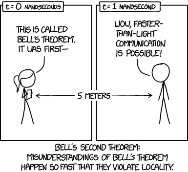
 |
| Source: xkcd.com/1591 |
I've also been told in person that I understood the theorem wrong. So it seems about time for some studying.
This time, rather than pick up Bell's original article, I read this more popular account of the argument, which covers more or less the same ground. If I understand it correctly, it's actually simpler than what I first thought, although my hazy understanding of the physics stood in the way of extracting the purely statistical part of the argument.
Background
Here's what I take to be the issue: We have a certain experiment in which two binary observables, $A$ and $B$, follow conditional distributions that depend on two control variables, $a$ and $b$:\begin{eqnarray}a &\longrightarrow& A \\
b &\longrightarrow& B
\end{eqnarray}Although the experiment is designed to prevent statistical dependencies between $A$ and $B$, we still observe a marked correlation between them for many settings of $a$ and $b$. This has to be explained somehow, either by postulating
- an unobserved common cause: $\lambda\rightarrow A,B$;
- an observed common effect: $A,B \rightarrow \gamma$ (i.e., a sampling bias);
- or a direct causal link: $A \leftrightarrow B$.
Measurable Consequences
The measure in question is the following:\begin{eqnarray}
C(a,b) &=& +P(A=1,B=1\,|\,a,b) \\
& & +P(A=0,B=0\,|\,a,b) \\
& & -P(A=1,B=0\,|\,a,b) \\
& & -P(A=0,B=1\,|\,a,b).
\end{eqnarray}This statistic is related to the correlation between $A$ and $B$ but different due to the absence of marginal probabilities $P(A)$ and $P(B)$. It evaluates to $+1$ if and only if the two are perfectly correlated, and $-1$ if and only if they are perfectly anti-correlated.
 |
| Contours of $C(a,b)$ when $A$ and $B$ are independent with $x=P(A)$ and $y=P(B)$. |
In a certain type of experiment, where $a$ and $b$ are angles of two magnets used to reveal something about the spin of a particle, quantum mechanics predicts that
$$
C(a,b) \;=\; -\cos(a-b).
$$When the control variables only differ little, $A$ and $B$ are thus strongly anti-correlated, but when the control variables are on opposite sides of the unit circle, $A$ and $B$ are closely correlated. This is a prediction based on physical considerations.
Bounds on Joint Correlations
However, let's stick with the pure statistics a bit longer. Suppose again $A$ depends only on $a$, and $B$ depends only on $b$, possibly given some fixed, shared background information which is independent of the control variables. |
| The statistical situation when the background information is held constant. |
Then $C(a,b)$ can be expanded to
\begin{eqnarray}
C(a,b) &=& +P(A=1\,|\,a) \, P(B=1\,|\,b) \\
& & +P(A=0\,|\,a) \, P(B=0\,|\,b) \\
& & - P(A=1\,|\,a) \, P(B=0\,|\,b) \\
& & - P(A=0\,|\,a) \, P(B=1\,|\,b) \\
&=& [P(A=1\,|\,a) - P(A=0\,|\,a)] \times [P(B=1\,|\,b) - P(B=0\,|\,b)],
\end{eqnarray}that is, the product of two statistics which measure how stochastic the variables $A$ and $B$ are given the control parameter settings. Using obvious abbreviations,
$$
C(a,b) \; = \; (A_1 - A_0) (B_1 - B_0),
$$and thus
\begin{eqnarray}
C(a,b) + C(a,b^\prime) &=&
(A_1 - A_0) (B_1 - B_0 + B_1^\prime - B_0^\prime)
& \leq & (B_1 - B_0 + B_1^\prime - B_0^\prime); \\
C(a^\prime,b) - C(a^\prime,b^\prime) &=& (A_1^\prime - A_0^\prime) (B_1 - B_0 - B_1^\prime + B_0^\prime)
& \leq & (B_1 - B_0 - B_1^\prime + B_0^\prime).
\end{eqnarray}It follows that
$$
C(a,b) + C(a,b^\prime) + C(a^\prime,b) - C(a^\prime,b^\prime) \;\leq\; 2(B_1 - B_0) \;\leq\; 2.
$$Since $(B_1 - B_0)\geq-1$, a similar derivation shows that
$$
| C(a,b) + C(a,b^\prime) + C(a^\prime,b) - C(a^\prime,b^\prime) | \;\leq\; 2|B_1 - B_0| \;\leq\; 2.
$$In fact, all 16 variants of this inequality, with the signs alternating in all possible ways, can be derived using the same idea.
Violations of Those Bounds
But now look again at$$
C(a,b) \;=\; -\cos(a-b).
$$We then have, for $(a,b,a^\prime,b^\prime)=(0,\pi/4,\pi/2,-\pi/4)$,
$$
\left| C\left(0, \frac{\pi}{4}\right) + C\left(0, -\frac{\pi}{4}\right) + C\left(\frac{\pi}{4}, \frac{\pi}{4}\right) - C\left(\frac{\pi}{4}, -\frac{\pi}{4}\right) \right| \;=\; -2\sqrt{2},
$$which is indeed outside the interval $[-2,2]$. $C$ can thus not be of the predicted functional form and at the same time satisfy the bound on the correlation statistics. Something's gotta give.
Introducing Hidden Variables
This entire derivation relied on $A$ and $B$ depending on nothing other than their own private control variables, $a$ and $b$.However, suppose that a clever physicist proposes to explain the dependence between $A$ and $B$ by postulating some unobserved hidden cause influencing them both. There is then some stochastic variable $\lambda$ which is independent of the control variables, yet causally influences both $A$ and $B$.
 |
| The statistical situation when the background information varies stochastically. |
However, even if this is the case, we can go through the entire derivation above, adding "given $\lambda$" to every single step of the process. As long as we condition on a fixed value of lambda, each of the steps still hold. But since the inequality thus is valid for every single value of $\lambda$, it is also valid in expectation, and we can thus integrate $\lambda$ out; the result is that even under such a "hidden variable theory," the inequality still holds.
Hence, the statistical dependency cannot be explained by a shared cause alone, since the functional form of the probability densities for $A$ given $a$ and $B$ given $b$ are of a wrong form. We will therefore need to either postulate direct causality between $A$ and $B$ or an observed downstream variable (sampling bias) instead.
Note that the only thing we really need to prove this result is the assumption that the probability $P(A,B \, | \, a,b,\lambda)$ factors into the product $P(A \, | \, a,b,\lambda)\, P(B \, | \, a,b,\lambda)$. This corresponds to the assumption that there is no direct causal connection between $A$ and $B$.