Billsingley: Ergodic Theory and Information (1965), pp. 12–14

In the process of proving the ergodic theorem, Billingsley also provides in passing a proof for a weaker theorem related to mixing operations: This states that for a class of processes that satisfy a certain limiting independence condition, visiting frequencies converge to probabilities.

Definitions

More precisely, a time shift $T$ is said to be mixing (p. 12) if$$
P(A \cap T^{-n}B)  \;  \rightarrow  \;  P(A)P(B)
$$for all sets $A$ and $B$. The process is thus mixing if information about the present is almost entirely independent of the far future. (A sample path $\omega$ belongs to the set $T^{-n}B$ if $\omega$ will visit $B$ after $n$ time shifts forward.) Billsingley doesn't comment on the choice of the term "mixing," but I assume it should be read as an ill-chosen synonym for "shuffling" in this context.

We will now be interested in the behavior of the visiting frequencies$$
P_n(A) \; := \;  \frac{1}{n} \sum_{k=0}^{n-1} \mathbb{I}_A(T^k\omega),
$$where $\mathbb{I}_A$ is the indicator function of some bundles of sample paths. This quantity is a random variable with a distribution defined by the distribution on the sample paths $\omega$.

Note that the traditional notion of visiting frequency (i.e., how often is the ace of spades on top of the deck?) is a special case of this concept of visiting frequency, in which the bundle $A$ is defined entirely in terms of the 0th coordinate of the sample path $\omega = (\ldots, \omega_{-2}, \omega_{-2}, \omega_{0}, \omega_{1}, \omega_{2}, \ldots)$. In the general case, the question of whether $\omega\in A$ could involve information stored at arbitrary coordinates of $\omega$ (today, tomorrow, yesterday, or any other day).

Theorem and Proof Strategy

The mixing theorem now says the following: Suppose that $P$ is a probability measure on the set of sample paths, and suppose that the time shift $T$ is mixing and measure-preserving with respect to this measure. Then$$
P_n(A)  \;  \rightarrow  \;  P(A)
$$in probability.

The proof of this claim involves two things:

1. Showing that $E[P_n(A)] = P(A)$;
2. Showing that $Var[P_n(A)] \rightarrow 0$ for $n \rightarrow \infty$.

These two assumptions collectively imply convergence in probability (by Markov's inequality).

Identity in Mean

The time shift $T$ is assumed to preserve the measure $P$. We thus have $$
E[f(\omega)] \; = \; E[f(T\omega)] \; = \; E[f(T^2\omega)] \; = \; \cdots
$$for any measurable function $f$. It follows that$$
E[\mathbb{I}_A(\omega)] \; = \;
E[\mathbb{I}_A(T\omega)] \; = \;
E[\mathbb{I}_A(T^2\omega)] \; = \; \cdots
$$and that these are all equal to $P(A)$. By the linearity of expectations, we therefore get that $E[P_n(A)] = P(A)$.

This proves that $P_n(A)$ at least has the right mean. Convergence to any other value than $P(A)$ is therefore out of the question, and it now only remains to be seen that the variance of $P_n(A)$ also goes to 0 as $n$ goes to infinity.

Vanishing Variance: The Idea

Consider therefore the variance$$
Var[P_n(A)]  \; = \;  E\left[ \left(P_n(A) - P(A)\right)^2 \right].
$$In order to expand the square under this expectation, it will be helpful to break the term $P(A)$ up into $n$ equal chunks and then write the whole thing as a sum:$$
P_n(A) - P(A)  \; = \;  \frac{1}{n} \sum_{k=0}^{n-1} (\mathbb{I}_A(T^k\omega) - P(A)).
$$If we square of this sum of $n$ terms and take the expectation of this expasion, we will get a sum of $n^2$ cross-terms, each of which are expected values of the form$$
Cov(i,j)  \; := \;  E\left[ \left(\mathbb{I}_A(T^i\omega) - P(A)\right) \times \left (\mathbb{I}_A(T^j\omega) - P(A)\right) \right].
$$By expanding this product and using that $E[\mathbb{I}_A(T^k\omega)]=P(A)$, we can find that$$
Cov(i,j)  \; = \;  E\left[\mathbb{I}_A(T^i\omega) \times \mathbb{I}_A(T^j\omega)\right] - P(A)^2.
$$The random variable $\mathbb{I}_A(T^i\omega) \times \mathbb{I}_A(T^j\omega)$ takes the value 1 on $\omega$ if and only if $\omega$ will visit $A$ after both $i$ and $j$ time steps. Hence,$$
Cov(i,j)  \; = \;  P(T^{-i}A \cap T^{-j}A)  -  P(A)^2,
$$and we can write$$
Var[P_n(A)]  \; = \;  \frac{1}{n^2} \sum_{i=0}^{n-1} \sum_{j=0}^{n-1} Cov(i,j).
$$The goal will now be to show the sum of these $n \times n$ converges to $0$ as we increase $n$.

Vanishing Variance: The Steps

Since $T$ is assumed to be measure-preserving, the value of $Cov(i,j)$ is completely determined by the distance between $i$ and $j$, not their absolute values. We thus have$$
Cov(i,j)  \; = \;  Cov(n+i, n+j)
$$for all $i$, $j$, and $n$.

By the mixing assumption, $Cov(0,j) \rightarrow 0$ for $j \rightarrow \infty$. Together with the observation about $|i-j|$, this implies that $$Cov(i,j) \;\rightarrow\; 0$$ whenever $|i-j| \rightarrow \infty$. If we imagine the values of  $Cov(i,j)$ tabulated in a huge, square grid, the numbers far away from the diagonal are thus tiny. We will now sum up the value of these $n^2$ numbers $Cov(i,j)$ by breaking them into $n$ classes according to the value of $d = |i-j|$.

To do so, we upper-bound the number of members in each class by $2n$: There are for instance $n$ terms with $|i-j|=0$, and $2(n-1)$ terms with $|i-j|=1$. (This upper-bound corresponds graphically to covering the $n\times n$ square with a tilted $n\sqrt{2} \times n\sqrt{2}$ square, except for some complications surrounding $d=0$.)

We thus have$$
Var[P_n(A)]
\; = \;
\frac{1}{n^2} \sum_{i=0}^{n-1} \sum_{j=0}^{n-1} Cov(i,j)
\;  \leq  \;
\frac{2}{n} \sum_{d=0}^{n-1} Cov(0,d).
$$This last quantity is an average of a list of numbers that converge to $0$; this average itself must therefore also converge to $0$ as $n\rightarrow \infty$. This proves that$$
Var[P_n(A)]  \; \rightarrow \;  0]
$$for $n \rightarrow \infty$, and we can conclude that $P_n(A) \rightarrow P(A)$ in probability.

Applicability

Note that this mixing assumption is very strong. A periodic Markov chain, for instance, will usually not be mixing: Consider for instance a process that alternates between odd and even values; the the joint probability $P(evens \cap T^n odds)$ will alternate between 0 and 1 as $n$ runs through the natural numbers. In many cases of practical interest, we therefore do in fact need the increased generality of the classic ergodic theorem.

Billingsley: Probability and Measure, Ch. 1.4

Prompted by what I found to be quite confusing about Patrick Billingsley's presentation of Kolmogorov's zero-one law, I've been reflecting a bit on the essence of the proof, and I think I've come to a deeper understand of the core of the issue now.

The theorem can be stated as follows: Let $S$ be an infinite collection of events equipped with a probability measure $P$ (which, by Kolmogorov's extension theorem, can be defined exhaustively on the finite subsets of $S$). Suppose further that $A$ is some event in the $\sigma$-extension of $S$ which is independent of any finite selection of events from $S$. Then $A$ either has probability $P(A)=0$ or $P(A)=1$.

The proof is almost evident from this formulation: Since $A$ is independent of any finite selection of events from $S$, the measures $P(\,\cdot\,)$ and $P(\,\cdot\,|\,A)$ coincide on all events that can be defined in terms of a finite number of events from $S$. But by Kolmogorov's extension theorem, this means that the conditional and the unconditional measures extend the same way to the infinite collection. Hence, if P$(A)>0$, this equality also applies to $A$, and thus $P(A\,|\,A)=P(A)$. This implies that $P(A)^2=P(A)$, which is only satisfied by $P(A)=1$.

So the core of the proof is that independence of finite selections implies independence in general. What makes Billingsley's discussion of the theorem appear a bit like black magic is that he first goes through a series of steps to define independence in the infinite case before he states the theorem. But this makes things more murky than they are in Kolmogorov's own statement of the theorem, and it hides the crucial limit argument at the heart of the proof.

An example of a "tail event" which is independent of all finite evidence is the occurrence of infinitely many of the events $A_1, A_2, A_3, \ldots$. The reasons that this is independent of an event $B \in \sigma(A_1, A_2, \ldots, A_N)$ is that$$
\forall x\geq 1 \, \exists y\geq x \, : A_y
$$is logically equivalent to$$
\forall x\geq N \, \exists y\geq x \, : A_y.
$$Conditioning on this some initial segment thus does not change the probability of this event.

Note, however, that this is not generally the case for events of the type$$
\forall x\geq 1 \, \exists y\geq 1 \, : A_y.
$$It is only the "$y\geq x$" in the previous case that ensures the equivalence.

A statement like "For all $i$, $X_i$ will be even" is for instance not a tail event, since a finite segment can show a counterexample, e.g., $X_1=17$. Crucially, however, this example fails to be a tail event because the events "$X_i is even$" (the inner quantification) can be written as a disjunctions of finitely many simple events. We can thus give a counterexample to the outer quantification ($\forall i$) by exhibiting a single $i$ for which the negation of "$X_i$ is even" (which is a universal formula) is checkable in finite time.

Reversely, if this were not the case for any of the statements in the inner loop, the event would be a tail event. That is, if the universal quantification were over a list of events which had no upper limit on the potential index of the verifier, then finite data could not falsify the statement. This happens when the existence of a single potential verifier implies the existence of infinitely many (as it does in the case of "infinitely often" statements, since any larger $y$ is an equally valid candidate verifier).

Events of the form $\exists y: A_y$ are also not tail events, since they are not independent of the counterexamples $\neg A_1, \neg A_2, \neg A_3\ldots$. They are, however, independent of any finite selection of positive events (which do not entail the negation of anything on the list).

We thus have a situation in which sets at the two lowest levels of the Borel hierarchy can have probabilities of any value in $[0,1]$, but as soon as we progress beyond that in logical complexity, only the values 0 and 1 are possible.

Illustration by Yoni Rozenshein.

Oddly enough, this means that no probability theory is possible on complex formulas: When a probability measure is defined in terms of a set of simple events, then the $\Delta_2$ events always have probability 0 or 1. This property is conserved at higher orders in the hierarchy, since the quantifications that push us up the hierarchy are countable (and a countable union of null sets is a null set, by the union bound).

Note also that$$
\lim_{N\rightarrow \infty} \cup_{i=1}^{N} \cap_{j=1}^{N} A_{ij}
\;=\;  \cup_{i=1}^{\infty} \cap_{j=1}^{\infty} A_{ij},
$$and since $$
P\left( \cup_{i=1}^{\infty} \cap_{j=1}^{\infty} A_{ij} \right)  \;\in\;  \{0,1\},
$$the probabilities of the finite approximations must converge to these extremes. As we spend more computational power checking the truth of a tail event on a specific sample, we thus get estimates that approach 0 or 1 (although without any general guarantees of convergence speed).

This sheds some light on what the theorem actually means in practice, and how it relates to the zero-one theorem for finite models of first-order logic.

Billingsley: Probability and Measure (1979), ch. 2

In the chapter on probability measures, Patrick Billingsley points out a potential fallacy that I can see that I have been making (pp. 24–25).

I have been thinking about the $\sigma$-field generated by a system $S$ as the limit of a series of $\sigma$-operations such as complements and countable unions. Such a recursive procedure for generating $\sigma(S)$ fails to generate all the required sets when, as I tacitly imagined, it is applied only countably many times.

This can be seen by means of a clever diagonal argument which involves constructing a bijection between the sets thus generated and the real unit interval. The gist of the proof is that when we only use countably many recursive steps, we can enumerate the resulting sets by means of sequences of integers, and this leaves the construction open to a diagonal counterexample.

The Playing Field

Let's first agree on a canonical defition of the Borel field $\mathcal{B}$ over $(0,1]$: For the present purposes, we will identify it as the $\sigma$-field generated by the intervals with rational endpoints, including the empty set.

This seed set $S$ is countable and can therefore be enumerated, for instance as

$\emptyset$, $(0,1]$, $(0,\frac{1}{2}]$, $(\frac{1}{2},1]$, $(0,\frac{1}{3}]$, $(\frac{1}{3},\frac{1}{2}]$, $(\frac{1}{3},1]$, $(0,\frac{1}{4}]$, $(\frac{1}{4},\frac{1}{3}]$, $(\frac{1}{4},\frac{1}{2}]$, …

For the purposes of this argument, let's further restrict the permitted $\sigma$-operations to

1. complementation;
2. countable unions.

These two operations can compactly be described as an application of the function
$$
\Psi(A_1,A_2,A_3,A_4,\ldots)\;=\; A_1^c \cup A_2 \cup A_3 \cup A_4 \cup \ldots
$$to a countable sequence of sets. We can then translate
\begin{eqnarray}
A^c &=& A^c \cup \emptyset \cup \emptyset \cup \emptyset \cup \emptyset \ldots \\
\cup_{i=1}^{\infty}A_i &=& \emptyset \cup A_1 \cup A_2 \cup A_3 \cup \ldots
\end{eqnarray}Any $\sigma$-operation is then a matter of applying $\Psi$ to some countable sequence of sets.

The Elements of Construction

This allows us to describe our inductive procedure in terms of a recursive function $R$ that uses $\Psi$ as a subroutine. We define the base case as a projection:
$$
R_0(A_1,A_2,A_3,\ldots) \;=\; A_1.
$$In order to define the recursion step, we first need to recall that $\mathbb{N}$ and $\mathbb{N}\times \mathbb{N}$ are equipotent, as can be seen from the following array:
$$
\begin{array}{ccccc}
1 & 2 & 4 & 7 & \ldots \\
3 & 5 & 8 & 12 & \ldots \\
6 & 9 & 13 & 18 & \ldots \\
10 & 14 & 19 & 25 & \ldots \\
\vdots & \vdots & \vdots & \vdots &
\end{array}

$$This array can be used to map a countable sequences of sets onto a countable sequence of countable sequences. We use this unraveling trick for the recursive step:
$$
R_n(A_1,A_2,\ldots) \;=\; \Psi( R_{n-1}(A_1,A_2,A_4,\ldots), R_{n-1}(A_3,A_5,A_8,\ldots), \ldots )
$$This way, we can, by a careful selection of rational intervals $A_1,A_2,A_3,\ldots$, select any countable sequence of $R_{n-1}$-sets we like and feed that sequence into a new $\Psi$-construction.

This trick, then, transforms a sequence of rational intervals into an $R_n$-set. In other words, any level $n$ set can be obtained in a (nominally) single step by feeding an appropriate sequence of level 0 sets into the recursive function $R_n$.

From Sequences to Sets

We now finally put
$$
R(A_1,A_2,\ldots) \;=\; R_1(A_1,A_2,\ldots) \cup R_2(A_3,A_5,\ldots) \cup R_3(A_6,A_9,\ldots) \cup \ldots
$$This format covers all sets that can be obtained by any finite level of recursion.

For instance, if a set can be produced by level 17 recursion, we can choose the sequence $A_1,A_2,A_3,\ldots$ so that all $R_i$ except $R_{17}$ return the empty set, while $R_{17}$ returns the set we are interested in. This is achieved by constructing the sequence $A_1,A_2,A_3,\ldots$ so that it splits into just the right subsequences.

In other words, we now have a method for picking out any set that requires only finite recursion by specifying an appropriate sequence of rational intervals. Since there are only countably many rational intervals, the selection of a specific finite-level recursive set is therefore a matter of selecting an appropriate sequence of natural numbers.

Stone to Stone

The set of countably infinite sequences of positive integers is equipotent with the real unit interval.

Specifically, Billingsley suggests that we use the bijection $b$ which for its $k$th integer takes the distance between the $(k-1)$st and the $k$th occurrence of the digit 1 in the binary expansion of the number $\omega\in(0,1]$.

Under this bijection,
$$
b\left(\frac{1}{3}\right) \;=\; b\left(.010101\ldots\right) \;=\; (2,2,2,2,\ldots).
$$For this definition to work, there has to be infinitely many 1s in the binary expansion. This can be guaranteed by always choosing the non-terminating binary expansion of $\omega$, so that, for instance,
$$
b\left(\frac{1}{2}\right) \;=\; b\left(.111111\ldots\right) \;=\; (1,1,1,1,\ldots).
$$Incidentally, this choice also fixes the ambiguity problems we might otherwise have, making $b$ a true bijection.

Because of the construction above, the output of this function can be fed into another function that translates the infinite sequences of integers into an infinite sequence of rational intervals, which is then translated into a recursive set. In other words, we can map any real number $\omega\in(0,1]$ onto a finite-recursion set $s(\omega)$. This establishes a surjection of the real numbers into the system of sets that can be obtained by finitely many $\sigma$-operations on the rational intervals.

The Diagonal

The set we now need for our diagonal counterargument is
$$
B = \{\omega\in (0,1]: \omega \not\in s(\omega)\}.
$$This set cannot be obtained by finite application of $\sigma$-operations to the rational intervals.

If it could, there would be at least one $\omega_0\in (0,1]$ such that $B=s(\omega_0)$. But by construction, $\omega_0\in s(\omega_0)$ holds if and only if $B\not \in s(\omega_0)$; so $B$ and $s(\omega_0)$ must disagree at least about the element $\omega_0$ and possibly about others. This contradicts the assertion that $B=s(\omega_0)$. Hence, $B$ cannot be obtainable by a finite number of recursive operations.

On the other hand, $B$ is a Borel set. Billingsley gives a complicated argument for this which is a notational nightmare, but I think he is just expressing a proof by induction.

Proof Sketch

The first step of the argument introduces a building block called $D_k$. This is the set of real numbers that are members of $A_k(\omega)$, the $k$th interval on their own list. For instance, $\omega=1/3$ is mapped onto the constant interval list
$$
(0,1], (0,1], (0,1], (0,1], \ldots
$$since $b(1/3)=(2,2,2,\ldots)$, and $(0,1]$ is the second interval on the list. It thus follows that $1/3\in A_k(1/3)$ for all $k$, and thus $1/3 \in D_k$ for all $k$.

The sets $D_k$ are Borel sets. This follows from the fact that the set of binary numbers with a specific $k$th waiting time is a Borel set, and that any rational interval is a Borel set.

The second part of the argument uses a translation between the set
$$
R_n(A_{m_1}(\omega), A_{m_2}(\omega), A_{m_3}(\omega), \ldots)
$$and the set
$$
R_n(D_{m_1}, D_{m_2}, D_{m_3}, \ldots)
$$for an arbitrary integer sequence $m_1, m_2, m_3, \ldots$. This equality is proven by induction.

Using this translation, the set $B^c = \{\omega\in s(\omega)\}$ can then be rewritten as a countable union of sets of this form. This shows that $B$ is indeed a Borel set, since the $D_k$ are.

A note on the Kolmogorov-Dynkin extension theorem

I've been somewhat confused about Kolmogorov's extension theorem, the uniqueness theorem for stochastic processes, but this note by Cozma Shalizi cleared up things a little bit.

Here's the set-up: We have a universe of values, $\Omega$, and this gives rise to a universe of sample paths, $\Omega^\mathbb{N}$. This universe of sample paths can be equipped with a probability measure. Such a measure maps bundles of sample paths, $B \subseteq \Omega^\mathbb{N}$, onto probabilities.

The measure has to respect the usual restrictions, including countable additivity. However, it doesn't have to (and in fact can't) accept all bundles as inputs.

The set of measurable bundles is defined inductively on the basis of one-dimensional base cases and some recursive operations. Specifically, a bundle is measurable if it is

1. the preimage under a coordinate projection of some measurable set $A \subseteq \Omega$;
2. constructed out of other measurable bundles by means of complementation, finite intersection, or countable union.

These rules define a system $S$.

We could also define a smaller system, $S^{-}$, by only allowing finite unions. A bundle in this smaller system corresponds to a proposition about a finite-dimensional projection of the stochastic process. If we take the $\sigma$-algebra generated by the smaller system, we recover the full system, $\sigma(S^{-})=S$.

The content of the Daniell-Kolmogorov exention theorem can now be stated as follows: Suppose that two measures $P$ and $Q$ assign the same values to all bundles in $S^{-}$; then they assign the same values to all bundles in $S$. This is equivalent to saying that if two stochastic processes have the same distribution under any finite-dimensional projection, then they have the same distribution.

Not surprisingly, the proof involves some facts about the limit behavior of measures on increasing sets. Specifically, when a series of sets $B_1, B_2, B_3, \ldots$ converges to some limit set $B$ from below, then the measures $\mu(B_1), \mu(B_2), \mu(B_3), \ldots$ must converge to the limit $\mu(B)$. This implies the uniqueness of the infinite-dimensional extension of a set of finite-dimensional projections.

Here is the proof as given by Shalizi: Let $W$ be the set of bundles under which $P$ and $Q$ agree. Then by assumption, $S^{-} \subseteq W \subseteq S$. We want to show that $\sigma(S^{-}) = S  \subseteq W$. We do this by showing that $W$ is a Dynkin system, and that $S^{-}$ is closed under finite intersection, since this will allow us to use Dynkin's $\lambda$-$\pi$ theorem.

A Dynkin system is a system of sets which contains the whole universe, is closed under complementation, and closed under disjoint, countable unions (or equivalently: increasing, countable unions). The set agreement system $W$ satisfies these three properties, since

1. $P(\Omega^{\mathbb{N}})=Q(\Omega^{\mathbb{N}})=1$, so $P$ and $Q$ agree on the bundle consisting of all sample paths;
2. For any bundle $B\in W$, $$P(B^c)=1-P(B)=1-Q(B)=Q(B^c),$$ so if $P$ and $Q$ agree on on a bundle, they also agree on its complement;
3. Finally, if $P$ and $Q$ agree on every bundle in an increasing series of sets $B_1, B_2, B_3, \ldots $, then the two series $$P(B_1), P(B_2), P(B_3), \ldots$$ $$Q(B_1), Q(B_2), Q(B_3), \ldots$$must have the same limit. Hence, whenever $P$ and $Q$ agree on a list of increasing bundles, they thus also agree on the set-theoretic limit of that series.

Thus, $W$ is a Dynkin system. This means that it is large enough to contain all the additional sets we put into the system $S^{-}$ by closing it under $\sigma$-operations. In other words, $\sigma(S^{-}) \subseteq W$. We thus have both $S \subseteq W$ and $W \subseteq S$ (which is true by definition), and thus $W=S$.

Here's an intuitive version of that proof:

The system $S$ on which $P$ and $Q$ are defined must itself be defined by certain recursive operations: Every set in $S$ is constructed from a finite-dimensional base case using only well-behaved operations.

The properties of probability measures guarantee that we can match each of these constructions, operation for operation and step by step, by a corresponding axiom which enforces a certain unique result. Because of this parallelism between the construction of the sample space and the propagation of necessity, no measurable set in $S$ actually has any wiggle room when the bases cases are identical.

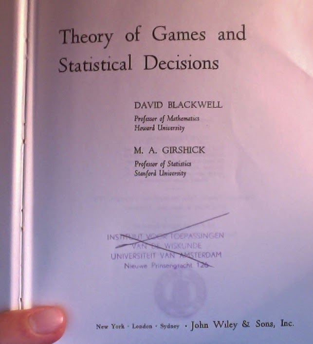
Blackwell and Girshick: Theory of Games and Statistical Decisions (1954), Ch. 4

There's an interesting representation theorem in Blackwell and Girshick's textbook in statistics: It provides a set of sufficient conditions for a preference ordering over lotteries to be expressible as a prior probability distribution (Th. 4.3.1, p. 118).

I assume the theorem comes from either Wald, Savage, or de Finetti, but no reference is given.

Well-Behaved Preferences

A lottery can here be defined as a function from the sample space to the real numbers. The conditions in the theorem are then the following:

• The ordering of two lotteries $f$ and $g$ cannot depend on the availability of other lotteries.
• If a lottery $f$ provides a higher payoff than a lottery $g$ at all points in the sample space $\Omega$, then $f$ must be preferred to $g$.
• If $f$ is preferred to $g$, then $f+h$ must be preferred to $g+h$.

An inspection of the proof also shows that they should have included a continuity condition:

• If $f_1, f_2, \ldots$ is a series of lotteries converging to a limit $f$, and if $f_i$ is preferred to $g$ for all $i$, then $f$ must also be preferred to $g$.

When these conditions are met, the preference ordering over the lotteries can be expressed as a distribution over the sample space, unless it categorizes all lotteries as equally good.

The Large and the Good

The proof of the theorem uses the fact that two convex, disjoint, open sets can be separated by a hyperplane. Here's a sketch:

If we let $e$ be the lottery that pays zero in all situations $\omega \in \Omega,$ then we can define the following sets:
\begin{eqnarray}
F[>] &=& \{f\ |\ \forall \omega \in \Omega: f(\omega) > 0\},
\\
F[\gtrsim] &=& \{f\ |\ f\gtrsim e\},
\end{eqnarray}
and we can further define, in the usual way, $F[>] + F[\gtrsim]$ to be the sums of lotteries from those two sets.

Now, $F[>]$ is an open set, and hence $F[>] + F[\gtrsim]$ is, too. Further, $F[>]$ and $F[\gtrsim]$ are both closed under addition (due to the third assumption), and hence their sum is, too. They are also both closed under multiplication with a scalar, and again, so is their sum — but this latter argument requires a bit more spelling out.

Rational and Real Convexity

Suppose a lottery $f$ is preferred to the zero lottery, that is, $f \in F[\gtrsim]$. The third assumption of the theorem then tells us that
$$
e \;\lesssim\; f \;\lesssim\; f + f \;\lesssim\; f + f + f \;\lesssim\; \ldots \;\lesssim\; nf.
$$
By further adding multiple copies of the zero lottery to both sides of this preference ineqality, we can see that
$$
me \;\lesssim\; (m-1)e + nf \;=\; nf,
$$
where we have selectively used the fact that $e$ is the zero lottery. Putting these facts together, we then have the preference inequality
$$
e \;\lesssim\; \left(\frac{n}{m}\right)f.
$$
By using a positive sequence of rational approximations $(n/m) \rightarrow \lambda$, we can use this fact along with the continuity assumption to conclude that $F[\gtrsim]$ is closed under multiplication with any positive, real scalar $\lambda$.

I don't think there's a way around this last technicality. It is, incidentally, the same proof technique used to prove that the logarithmic functions are the only continuous functions that turn products into sums.

Cutting the Cake

At any rate, $F[>] + F[\gtrsim]$ is an open and convex set separated from the singleton set $\{e\}$. We can therefore conclude that there is a lottery (or vector) $p$ which defines the hyperplane $\{f\ |\ f\cdot p=0\}$ separating $F[>] + F[\gtrsim]$ from $\{e\}$. The set $F[>] + F[\gtrsim]$ is thus a subset of the half-space $\{f\ |\ f\cdot p \geq 0\}$.

This vector $p$ must have nonnegative coordinates, since the set $F[>]$ is unbounded in all positive directions. If $p$ had a negative coordinate, $p(\omega) \leq 0$, we could choose a lottery for which the corresponding coordinate, $f(\omega)$, was so large that $f\cdot p < 0$. This would violate the definition of $p$, and $p$ hence has to be a nonnegative vector which can be interpreted as a probability distribution.

It would also have the property that $f\cdot p \geq g\cdot p$ if and only if $f \gtrsim g$. This follows from the fact that $f\cdot p \geq g\cdot p$ if and only if $(f - g) \in F[>] + F[\gtrsim]$, which holds if and only if $f$ can be expressed as the sum of $g$ and some lottery preferable to the zero lottery.

Cardano: The Book on Games of Chance (1961/1663)

Cardano; from Wikimedia.

My library has refused to buy the new translation of Jacob Bernoulli's Ars Conjectandi (1713), possibly because the price tag is on the order of $3000. Consequently, I don't have an English translation of the complete book, arguably the most influential one in the history of probability (perhaps with the exception of Kolmogorov's little pamphlet).

Meanwhile, they hold two copies of Cardano's weird, chatty, and uneven book on gambling. I checked out both of them, only two find out that one (the 1961 version) was a reprint of the other, the translation by Øystein Ore appended to his own 1953 commentary on the book (which, incidentally, also included an interpretation of Cardano's erroneous calculus of probabilities).

I'll deal with Ore's book later. Now a few comments on quotes on Cardano.

Contents

Cardano's book can roughly be divided up into sections as follows. If it looks jumbled up, it's because it is.

• Chapters 1–10: Preliminaries, survey of games, moralistic preaching, etc.
• Chapters 9–11: Combinatorics of dice games.
• Chapters 16–19: On card games (mostly non-mathematical discussions of cheating, moral issues, and the like).
• Chapters 20–21: On luck.
• Chapters 22–25: More game taxonomies and definitions.
• Chapter 26: On theoretical and practical knowledge.
• Chapter 27: More on luck
• Chapter 28: Recommendations on playing styles in backgammon.
• Chapter 29: On why you shouldn't play against hotheads.
• Chapters 30–31: Games in ancient Greece.
• Chapter 32: Computing expectations for a die.

From the perspective of the history of mathematics proper, the most directly relevant parts are those on combinatorics and those on luck.

"If Fortune Be Equal"

One of the more remarkable features of Cardano's book is the prominent place it gives to "luck." As Lorraine Daston has noted, this concept seemed to fill out any gap his calculus didn't account for, including the gap between frequencies and probabilities, or between expectations and actual outcomes.

Mean playing dice; illustration from a 1531 print of Cicero's On Duties.

The first time the word occurs is during Cardano's dicussion of fair bets. Apparently, the most common dice game at the time was a bet on whether a specific throw (e.g., double six) would show up or not show up within n throws of a number of dice.

Cardano was therefore interested in computing the number n for which this bet would be fair — or in his words, for which "there is equality." He explains in Chapter 11:

This gives eighteen casts for equality for a throw (1,1); for in that number of casts this throw can appear and not appear with equal probability; and similarly for the throws (2,2) and (3,3).

But the throw (1,2) can turn up in two ways, so that for it there is equality in nine casts; and if it turns out up more frequently or more rarely, that is a matter of luck. (p. 11; my emphasis)

Later, in Chapter 14:

If, therefore, someone should say, "I want an ace, a deuce, or a trey," you know that there are 27 favorable throws, and since the [size of the] circuit [= sample space] is 36, the rest of the throws in which these points will not turn up will be 9; the odds will therefore 3 to 1.

• Therefore in 4 throws, if fortune be equal, an ace, deuce, or trey will turn up 3 times and only one throw will be without any of them;
• if therefore, the player who wants an ace, deuce, or trey were to wager three ducats and the other player one, then the former would win three times and would gain three ducats; and the other once and would win three ducats;
• therefore in the circuit [= observation] of 4 throws they would always be equal. (p. 16; my epmhasis; my itemization)

His language use here suggests that, on some level, he believes that the expected values must somehow be realized — they are what the game should pay off if it weren't for all these kinks and imperfections in the universe.

"The Length of Time … shows Forth All Forms"

Apparently, he is completely serious about this. In a later chapter on skill (ch. 27), he lists two "methods" by which fortunes can change, the second being the more occult one:

But of the other method there is also some secret principle. To these matters belong amulets, witchcraft, and the like, and just as in each case (as they say) the sword fits its own sheath and the foot its own show, so the hour, the day, the year, and the place must fit; so also in this question, what will make one man happy will make another wretched. (p. 44)

Austrian 16th century woodcut of two soldiers playing dice.

Cardano does seem to think, however, that time tends to cancel out luck. In the chapter on sequential successes, he computes the probability of observing an unbroken string of 20 repetitions of a probability 1/2 event, wrongly getting the answer to be 1/8000. He comments:

Yet it can scarcely be believed that in 7,999 throws a player can cast an even number twenty times in a row. But we have demonstrated this; because, although in 8,000 performed only once, this reasoning can deceive us, still in an infinite number of throws, it is almost necessary for it to happen; for the magnitude of the circuit is the length of time which shows forth all forms. (pp. 19–20).

Here, "luck" almost seems to be synonymous with "noise."

Squares and Cubes

Since I'm talking about this error anyway, and since this is essentially the sole remaining mathematical component of the book, let me just quickly summarize what Cardano seems to be doing in the rest of Chapters 14 and 15.

At the end of Chapter 14, he claims that if the odds in favor of a single success is p : 1 – p, then odds in favor of k successes in a row are p^k : (1 – p)^k. This is not correct, since (1 – p)^k is not in general equal to 1 – p^k. He recognizes this in the opening of Chapter 15, noting that if it were really true, any run of consecutive probability 1/2 events would also have probability 1/2:

But this reasoning seems to be false, even in the case of equality, as, for example, the chance of getting one of any three chosen faces in one cast of one die is equal to the chance of getting one of the other three, but according to this reasoning there would be an even chance of getting a chosen face each time in two casts, and thus in three, and four, which is most absurd. For if a player with two dice can with equal chances throw an even and an odd number, it does not follow that he can with equal fortune throw an even number in each of three successive casts. (p. 19)

 Cardano 1 

 Cardano 2  

Correct 

1 : 1

1 : 1

1 : 1

1 : 1

3 : 1

3 : 1

1 : 1

8 : 1

7 : 1

1 : 1

15 : 1

15 : 1

1 : 1

24 : 1

31 : 1

1 : 1

35 : 1

63 : 1

1 : 1

48 : 1

123 : 1

So now Cardano owes us a different argument. He therefore goes on to claim that the correct answer for p = 1/2 in fact is k² – 1 : 1. This coincides with the correct answer for a couple of small values, but then diverges exponentially from it. This leads him to make the "infinity" remark quoted above.

Parenthetically, I'm not sure why he would cube rather than square the number 20 in that example. Perhaps Ore has something intelligent to say about this.

Late 15th century book illustration showing a dice game.

How To Gamble If You Must

In Chapter 20, Cardano tells a little autobiographical anecdote as an illustration of his points about fortune, luck, etc. This story is not strictly relevant to my topic here, but it is simply to bizarre not to quote. Hence, Ladies and Gentlemen, Cardano without filter:

Yet I have decided to submit to the judgment of my readers what happened to me in the year 1526 in the company of Thomas Lezius, the patrician of Venice, leaving it to each reader to form his own opinion. I had just duly resigned from the office of rector of the scholars in the University of Padua on the third of August, and now I was journeying with Hieronymus Rivola, a scholar from Bergamo, on a certain night of the same month toward Venice. We were playing a game (called Bassette) and I won all the money he had. Then he asked me to play with him on credit, if I am not mistaken up to two or three aurei, and I won again. Then, finally, he wanted to carry it on endlessly, but I refused. He promised to pay what he owed me within three ways; he did not come.

Then he chanced to meet me and said that he would come to pay the money on Saturday (which was the day of the Nativity of the Virgin) and promised to take me to a beautiful prostitute. At that time I was just completing my twenty-fifth year, but I was impotent. Nevertheless, I accepted the condition; there was not a word about the game. He came on the day agreed; and in that year the festival of the Blessed Virgin was on Saturday. He took me to the home of Thomas Lezius; there was no Thais there, but a bearded man with a young servant. No money was paid but we played with marked cards. I lost to him all the money which he owed me, and he reckoned it as part of his debts just as though he had given it to me. I list about twenty-five aurei or even a few more which I had, and played on, giving my clothes and my rings as security.

I returned home in sadness (as was natural), especially since there was no hope of getting money from home because uprisings and plots were raging at Milan. And so (and now I tell the truth, there being no reason why I should lie), I contrived for myself a certain art; I do not now remember what it was, since thirty-eight years have passed, but I think it took its rise in geomancy, by which I kept in mind on up to twenty-four plays all the numbers whereby I should win and all those whereby I should lose; by chance the former were far more numerous than the latter, even in the proportion (if I am not mistaken) of seven to one; and I do not recall now in what order these were against me.

But when I saw that I could not safely hold more numbers in my memory, I admonished my young servant, whose name was Jacob, that when he saw I had won back my clothes and my money he was to call me. I threatened that if he did not do it I would beat him severely. He promised and we went. As the game went on I won and lost in all the plays just as I had foreseen and after the third play I realized that there was no trickery or deceit about it. They laid down money freely and I accepted the wagers, but he was delighted be the example of the previous day and also on account of the marked cards (as I have said).

Thus his thoughts were inflamed by his youthful ardor; but the result was otherwise, for, on those plays in which I saw (as it were, without any real foreknowledge) that I would win, I did not rehect any amount of money and made large bets of my own, and in the other cases, where I knew he would win, I refused if he was the first to wager, and wagered very meagerly myself: thus the result was that within twenty plays I regained my clothes, my rings, and money and also what he had added besides. As for the clothes, the rings, and a collar for the boy, I sent them home piecemeal. Out of the total number there remained four deals; I played and won, and also came out victor in a few deals which were not contained in the number.

He was already perturbed and full of admiration, since he saw that in all the plays in which we played for high stakes I came out the victor, and in those in which he won I myself wagered little and when he wished to wager a great deal I refused. So (he said) I believe some demon is advising you, or that you know by some enchantment what is going to happen. What happened after that I remember that I have narrated elsewhere. (pp. 32–34)

He also gives a bit of extra detail in Chapter 17, the chapter on fraud in card games:

There are also some who smear the cards with soap so that they may slide easily and slip past one another. This was the trick practiced upon me by the well-known Thomas Lezius of Venice, patrician, when in my youth I was addicted to gambling. (p. 27)

Extraordinary, isn't it?

Fisher: Statistical Methods and Scientific Inference (1956), chapter 5.7

In chapter V of his book on statistical inference, Fisher compares various likelihood-based approaches to coming up with a predictive distribution. Some of the details are quite obscure, and I have problems following his argument in several places.

Section 2 is dedicated to to the Bayesian solution for a series of coin flips. It contains, among other things, a strange reference to coefficients other than the binomials, suggesting that these can be replaced freely with any other suitable polynomial (p. 112). I am not quite sure what he means or how he imagines this should be justified.

Section 7 is dedicated to a particular type of frequentist prediction. The set-up is that we have observed the counts a and b (heads and tails) and that we would like to find the likelihood of a continuation having counts c and d.

In order to find this, he suggests that we compute the likelihood ratio

Pr(a, b | f) Pr(c, d | f) / Pr(a + c, b + d | f).

The logic behind this computation is that a/b is close to c/d, then the joint probability of those two ratios is approximately the same as the probability of the pooled ratio (a + c)/(b + d). If, on the other hand, they both deviate highly from the maximum likelihood estimate (in different directions), then the joint probability will be lower than the pooled reference value. However, the actual value of the parameter of the coin flip cancels out from the fraction and thus plays no direct role in the computation.

Fisher goes through an example in which a = 3, b = 16, c = 14, d = 7. In order to compute the many factorials for this example, he uses the (very rough) approximation

x! ≈ x^x.

Or at least that's what I think he does — he comments that this x^x is "among others having the same margins," whatever that is supposed to mean (p. 129).

N! (green) and the approximation N^N (red).

At any rate, we can redo his computation using both his own approximate method and the exact formula, getting a likelihood of about .004 (Fisher's result) or .001 (the exact result).

As he suggests on page 130, we can also compile a table of likelihoods for various other values of c and d adding to 21. We can collect all of these results in a table like the following:

Count Fisher Exact Bayes 0 .094 .098 .048 1 .0499 .223 .109 2 .0836 .309 .151 3 .991 .336 .164 4 .964 .311 .152 5 .817 .256 .125 6 .621 .192 .094 7 .432 .133 .065 8 .277 .085 .042 9 .164 .051 .025 10 .090 .028 .014 11 .046 .015 .007 12 .022 .007 .003 13 .009 .003 .002 14 .004 .001 .001 15 .001 .000 .000 16 .000 .000 .000 … … … … Sum 5.867 2.050 1.000

As the table shows, the exact likelihoods coincide with the Bayes estimates if we normalize them. I think this is only the case because the numbers are large enough because of an issue with the normalizing constants in a Dirichlet distribution, but I don't have time to check the details now.

Arnauld: Logic (1662), Part IV, chs. 13–16

19th-century portrait of Arnauld, the main author of the Logic.

The last four chapters of the Port-Royal Logic deal with reasoning under uncertainty. They touch briefly on issues of evidential support, balanced odds, and fair games.

In retrospect, these remarks are difficult not to read as a precursors of later probability theory. Many authors have pointed this out, including Ian Hacking and Lorraine Daston.

I'm reading the 1996 translation by Jill Buroker, published by Cambridge UP.

The content of the four chapters on probability, or plausibility, are:

• Chapter 13, "Some Rules for directing reason well in beliefs about events that depend on human faith," argues that the standard of geometric proof and mathematical certainty only applies to matters of "immutable essence," and that judgment about human affairs should be made by meditating on the available evidence and testimonies.
• Chapter 14, "Application of the preceding rule to the beliefs about miracles," claims that this means that there are several instances in which it is reasonable to believe miracles took place, even if this cannot be proven beyond all reasonable doubt.
• Chapter 15, "Another remark on the same subject of beliefs about events," adds that this explains why certain deeds are attested by two notaries, and that the technique of weighing the evidence also has applications to authorship attribution for ancient (religious) manuscripts.
• Chapter 16, "The Judgments we ought to make concerning future events," argues that the doctrine not only applies to reasoning about the past, but also about the prediction of the future; a number of fair and unfair games are described as examples, and a version of Pascal's wager is then put forward.

Quotes follow below.

Don't Hold Your Breath

In chapter 13, we are told that the methodology of geometric proof works for geometry,

But if we try to use the same rules for beliefs about human events, we will always judge them falsely, except by chance, and we will make a thousand fallacious inferences about them. (p. 263)

Instead, we have to look for circumstantial evidence:

In order to decide the truth about an event and to determine whether or not to believe in it, we must not consider it nakedly and in itself, as we would a proposition of geometry. But we must pay attention to all the accompanying circumstances, internal as well as external. I call those circumstances internal that belong to the fact itself, and those external that concern the persons whose testimony leads us to believe in it. Given this attention, if all the circumstances are such that it never or only rarely happens that similar circumstances are consistent with the falsity of the belief, the mind is naturally led to think that it is true. Moreover, it is right to do so, above all in the conduct of life, which does not require greater certainty than moral certainty, and which even ought to be satisfied in many cases with the greatest probability.

But if, on the contrary, these circumstances are such that they are often consistent with the falsity of the belief, reason would require either that we remain in suspense, or that we view as false whatever we are told when its truth does not look likely, even if it does not look completely impossible. (p. 264)

Cloister of the Hôpital Cochin, inhabiting the former site of the Port-Royal abbey.

 

A Perversion of Reason

This idea is echoed in chapter 15:

Since we should be satisfied with moral certainty in matters not susceptible of metaphysical certainty, so too when we cannot have complete moral certainty, the best we can do when we are committed to taking sides is to embrace the most probable, since it would be a perversion of reason to embrace the less probable. (p. 270)

We also hear that negative evidence "weaken or destroy in the mind the grounds for belief" (p. 270).

A couple of things worth noting about these quotes:

• The process described here is a mental therapy, not a decision calculus; you pay close attention, and your "mind is naturally led" to a certain belief.
• The focus is on human affairs, that is, on practical matters.
• As in frequentist statistics, the contrast is not between true and false, but between confirmed and unconfirmed; we thus "remain in suspense" if the evidence is insufficient.

Set the Record Straight

Chapter 16 pours scorn on "many people" for entertaining a certain "illusion":

This is that they consider only the greatness and importance of the benefit they desire or he disadvantage they fear, without considering in any way the likelihood or probability that this benefit or disadvantage will or will not come about. (p. 273)

That is, thinking only of utility while ignoring probability. Moreover,

This is what attracts so many people to lotteries: Is it not highly advantageous, they say, to win twenty thousand crowns for one crown? Each person thinks he will be the happy person who will win the jackpot. No one reflects that if it is, for example, twenty thousand crows, it may be thirty thousand times more probable for each individual to lose rather than to win it.

The flaw in this reasoning is that in order to decide what we ought to do to obtain some good or avoid some harm, it is necessary to consider not only the good or harm itself, but also the probability that it will or will not occur, and to view geometrically the proportion all these things have when taken together. This can be clarified by the following example.

There are game in which, if ten persons each put in a crown, only one wins the whole pot and all the others lose. This each person risks losing only a crown and may win nine. If we consider only the gain and loss in themselves, it would appear that each person has the advantage. But we must consider in addition that if each could win nine crowns and risks losing only one, it is also nine times more probability for each person to lose one crown and not to win nine. Hence each has nine crowns to hope for himself, one crown to lose, nine degrees of probability of losing a crown, and only one of winning the nine crowns. This puts the matter at perfect equality. (pp. 273–74)

This argument is then pushed a little further to deal with some more extreme bets; to the fear of lightning, which is allegedly irrational and has to be "set straight" (p. 275); and finally to a version of Pascal's wager.

Jeffreys: Scientific Inference, third edition (1973)

This book, first published 1931, covers much of the same ground as Jeffreys' Theory of Probability (1939), but it's shorter and easier to read.

It touches on a number of extremely interesting topics, including

• the asymptotic equivalence of Bayesian inference and maximum likelihood inference (§4.3, pp. 73–74)
• a Bayesian notion of "statistical test" (§3.5, pp. 54–56)
• priors based on theory complexity (§2.5, especially pp. 34–39)
• the convergence of predictive distributions to the truth under (very) nice conditions (§2.5)
• an inductive justification of the principle of induction through hierarchical models (§3.7, pp. 58–60)
• a critique of the frequency theory of probability (§9.21, pp. 193–197)
• a number of other philosophical issues surrounding induction and probability (§9)

I might write about some of these issues later, but now I want to focus on a specific little detail that I liked. It's a combinatorical argument for Laplace's rule, which I have otherwise only seen justified through the use of Euler integrals.

Laplace's rule: Add a "virtual count" to each bucket before the parameter estimation.

The Generative Set-Up

Suppose that you have a population of n swans, r of which are white. We'll assume that r is uniformly distributed on 0, 1, 2, …, n. You now inspect a sample of m < n swans and find s white swans among them.

It then turns out that the probability that the next swan is white is completely independent of n: Whatever the size of the population is, the probability of seeing one more white swan turns out to be (s + 1)/(m + 1) when we integrate out the effect of r.

A population of n swans contains r white ones;
in a sample of m swans, s are white.

Let me go into a little more detail. Given n, m, and r, the probability of finding s white swans in the sample follows a hypergeometric distribution; that is,

Pr( s | n, m, r )  ==  C(r, s) C(n – r, m – s) / C(n, m),

where C(a, b) is my one-dimensional notation for the binomial coefficient "a choose b." The argument for this formula is that

• C(r, s) is the number ways of choosing s white swans out of a total of r white swans.
• C(n – r, m – s) is the number of ways of choosing the remaining m – s swans in the sample from the remaining n – r swans in the population.
• C(n, m) is the total number of ways to sample m swans from a population of n.

The numerator thus counts the number of ways to select the sample so that it respects the constraint set by the number s, while the denominator counts the number of samples with or without this constraint.

Inverse Hypergeometric Probabilities

In general, binomial coefficients have the following two properties:

• C(a, b) (a – b)  ==  C(a, b + 1) (b + 1)
• C(a + 1, b + 1)  ==  C(a, b) (a + 1)/(b + 1)

We'll need both of these facts below. They can be shown directly by cancelling out factors in the factorial expression for the binomial coefficients.

One consequence is that Bayes' rule takes on a particularly simple form in the hypergeometric case:

• Pr( r | n, m, s )  ==  Pr( s | n, m, r ) (m + 1)/(n + 1)
• Pr( s | n, m, r )  ==  Pr( r | n, m, s ) (n + 1)/(m + 1)
• Pr( s + 1 | n, m + 1, r )  ==  Pr( r | n, m + 1, s + 1 ) (n + 1)/(m + 1)

These equalities are, of course, saying the same thing, but I state all three forms because they will all come up.

By using the first of the two rules for binomial coefficients, we can also show that

Pr( s | n, m, r ) (r – s)/(n – m)  ==  Pr( s + 1 | n, m + 1, r ) (s + 1)/(n + 1)

According to the last fact about the inverse hypergeometric probabilities, this also means that

Pr( s | n, m, r ) (r – s)/(n – m)  ==  Pr( r | n, m + 1, s + 1 ) (s + 1)/(m + 1)

I have cancelled two occurrences of (n + 1) to arrive at this expression. I will use this fact below.

Expanding the Predictive Probability

By assumption, we have inspected s out of the r white swans, so there are r – s white swans left. We have further inspected m out of the n swans, so there is a total of n – m swans left. The probability that the next swan will be white is thus (r – s)/(n – m).

If we call this event q, then we have, by the sum rule of probability,

Pr( q | n, m, s )  ==   Σr Pr( q, r | n, m, s )

By the chain rule of probabilities, we further have

Pr( q | n, m, s )  ==   Σr Pr( q | n, m, s, r ) Pr( r | n, m, s )

As argued above, we have

• Pr( q | n, m, s, r ) = (r – s)/(n – m)
• Pr( r | n, m, s ) = Pr( s | n, m, r ) (m + 1)/(n + 1)
• Pr( s | n, m, r ) (r – s)/(n – m)  ==  Pr( r | n, m + 1, s + 1 ) (s + 1)/(m + 1)

Putting these facts together and cancelling, we get

Pr( q | n, m, s )  ==   (s + 1)/(m + 1) Σr Pr( r | n, m + 1, s + 1 )

I have pulled the constant factors out the summation here. Notice further that the summation is a sum of probabilities for the possible values of r. It must consequently sum to 1. We thus have

Pr( q | n, m, s )  ==   (s + 1) / (m + 1)

as we wanted to prove.

Carnap and Jeffrey: Studies in Inductive Logic and Probability, Vol. 1 (1971)

Carnap at his desk; from carnap.org.

This is an anthology edited by Rudolf Carnap and philosopher Richard C. Jeffrey (not to be confused with physicist Harold Jeffreys).

The majority of the book is dedicated to two essays on probability which Carnap intended to be a substitute for the (never realized) second volume of the Logical Foundations of Probability (1950). Carnap's idea is that rational belief should be understood as the result of probabilistic conditioning on a special kind of "nice" prior.

An Inconsistent Axiomatization of Rationality

In order to demarcate the realm of rational belief, Carnap has to specify the set of permitted starting states of the system and its update rules. He does so by means of the following four "rationality assumptions":

1. Coherence — You must conform to the axioms of probability; or in terms of gambling, you may not assign positive utility to any gamble that guarantees a strict loss.
2. Strict Coherence — You may not assign an a priori probability of 0 to any event; or equivalently, you may not assign positive utility to a gamble that renders a strict loss possible and a weak loss necessary.
3. Belief revision depends only on the evidence — Your beliefs at any time must be determined completely by your prior beliefs and your evidence (nothing else). Assuming axiom 1 is met, this comes down to producing new beliefs by conditioning.
4. Symmetry — You must assign the same probability to propositions of the same logical form, i.e., F(x) and F(y).

These axioms are inconsistent in a number of cases, and Carnap does not seem to realize. The problems are that

• Many infinite sets cannot be equipped with a proper, regular, and symmetric distribution. For instance, there is no "uniform distribution on the integers";
• There may be interdependent propositional functions in the language, and a prior that renders one symmetric might render another asymmetric. Consider for instance F(x) = "the box has a side-length between x and x + 1" and G(x) = "the box has a volume between x and x + 1".

Maybe Carnap had a vague idea about the first problem — at least he seems to assume that the sample space is finite throughout the first essay ("Inductive Logic and Rational Decisions," cf. pp. 7 and 14).

In the second essay, however, he explicitly says that there are countably many individuals in the language, so it would seem that he owes us a proper, coherent, and regular distribution on the integers ("A Basic System of Inductive Logic, Part I," ch. 9, p. 117).

Both Jaynes and Jeffreys made attempts at tackling the second problem by choosing priors that would decrease the tension between two descriptions. Jeffreys, for instance, showed that a probability density function of the form f(t) = 1/t (restricted to some positive interval) makes it irrelevant whether a normal distribution is described in terms of its variance or its precision parameter. Jaynes, by an essentially identical argument, "solved" Bertrand's paradox by choosing a prior that minimizes the discrepancy between a side-length description and a volume-description.

What is a Rationality Assumption?

Carnap knows that probability theory has to be founded on something other than probability theory to make sense and explains that "the reasons for our choice of the axioms are not purely logical." (p. 26; his emphasis).

Rather, they are game-theoretic: In order to argue against the use of some a priori probability measure (or "M-function"), Carnap must show why somebody starting from this prior

…, in a certain possible knowledge situation, would be led to an unreasonable decision. Thus, in order to give my reasons for the axiom, I move from pure logic to the context of decision theory and speak about beliefs, actions, possible losses, and the like. (p. 26)

That sounds circular, but the rest of his discussion seems to indicate that he is thinking about worst-case (or minimax) decision theory, which makes sense.

"Reduced to one"

What does not make sense, however, is his unfounded faith that there are always reasons to prefer one M-function over another:

Even on the basis of all axioms that I would accept at the present time …, the number of admissible M-functions, i.e., those that satisfy all accepted axioms, is still infinite; but their class is immensely smaller than that of all coherent M-functions [i.e., all probability measures]. There will presumably be further axioms, justified in the same way by considerations of rationality. We do not know today whether in this future development the number of admissible M-functions will always remain infinite or will become finite and possibly even be reduced to one. Therefore, at the present time I do not assert that there is only one rational Cr₀-function [= initial credence = credence at time 0]. (p. 27)

But clearly, he hopes so.

Carnap the Moralist

Interestingly, Carnap makes a very direct connection between moral character and epistemic habits. This comes out most clearly in a passage in which he explains that rationality is a matter of belief revision rather than belief:

When we wish to judge the morality of a person, we do not simply look at some of his acts; we study rather his character, the system of his moral values, which is part of his utility function. Observations of single acts without knowledge of motives give little basis for judgment. Similarly if we wish to judge the rationality of a person's beliefs, we should not look simply at his present beliefs. Information on his beliefs without knowledge of the evidence out of which they arose tells us little. We must rather study the way way in which the person forms his beliefs on the basis of evidence. In other words, we should study his credibility function, not simply his present credence function. (p. 22)

The "Reasonable Man" (to use the 18th century terminology) is thus the man who updates his beliefs in a responsible, careful, and modest fashion. Lack of reason is the stubborn rejection of norms of evidence, a refusal to surrender to the "truth cure."

As an illustration of what he has in mind, Carnap considers an urn example in which a person X observes a majority of black balls being drawn (E), and Y observes a majority of white balls (E'). He continues:

Let H be the prediction that the next ball drawn will be white. Suppose that for both X and Y the credence of H is 2/3. Then we would judge this same credence value 2/3 of the proposition H as unreasonable for X, but reasonable for Y. We would condemn a credibility function Cred as nonrational if Cred(H | E) = 2/3; while the result Cred(H | E') = 2/3 would be no ground for condemnation. (p. 22)

So although he elsewhere argues that rationality is a matter of risk minimization, he nevertheless falls right into the moralistic language of "grounds for condemnation."

Do the Robot

A similar formulation appears earlier, as he discusses the axiom that belief revision is based on evidence only. For a person satisfying this criterion, Carnap explains,

… changes in his credence function are influenced only by his observational results, but not by any other factors, e.g., feelings like his hopes or fears concerning a possible future event H, feelings that in fact often influence the beliefs of all actual human beings. (pp. 15–16)

 Like Jaynes, he defends this idealization by reference to a hypothetical design problem:

Thinking about the design of a robot might help us in finding rules of rationality. Once found, these rules can be applied not only in the construction of a robot but also in advising human beings in their effort to make their decisions as rational as their limited abilities permit. (p. 17)

Another way of saying the same thing is that we should first describe the machine that we would want to do the job, and then tell people how to become more like that machine.

Walters: An Introduction to Ergodic Theory (1982), p. 26

Book cover; from Booktopia.

Section 1.4 of Peter Walters' textbook on ergodic theory contains a proof of Poincaré's recurrence theorem. I found it a little difficult to read, so I'll try to paraphrase the proof here using a vocabulary that might be a bit more intuitive.

The Possible is the Necessarily Possible

The theorem states the following: If

1. X is a probability space
2. T: X → X is a measure-preserving transformation of X,
3. E is an event with positive probability,
4. and x a point in E,

then the series

x, Tx, T²x, T³x, T⁴x, …

will almost certainly pass through E infinitely often. Or: if it happens once, it will happen again.

The idea behind the proof is to describe the set R of points that visit E infinitely often as the superior limit of a series of sets. This description can then be used to show that E ∩ R has the same measure as E. This will imply that almost all points in E revisit E infinitely often.

Statement and proof of the theorem; scan from page 26 in Walters' book.

I'll try to spell this proof out in more detail below. My proof is much, much longer than Walters', but hopefully this means that it's much, much more readable.

Late Visitors

Let R_i be the set of points in X that visit E after i or more applications of T. We can then make two observations about the series R₀, R₁, R₂, R₃, …:

First, if j > i, and you visit E at a time later than j, you also visit E at a time later than i. The R_i's are consequently nested inside each other:

R₀ ⊃ R₁ ⊃ R₂ ⊃ R₃ ⊃ …

Let's use the name R for the limit of this series (that is, the intersection of the sets). R then consists of all the points in X that visit E infinitely often.

The series of sets is downward converging.

Second, R_i contains the points that visit E at time i or later, and the transformation T^–1 takes us one step back in time. The set T^–1R_i consequently contains the points in X that visit E at time i + 1 or later. Thus

T^–1R_i = R_{i + 1}.

But since we have assumed that T is measure-preserving, this implies that

m(R_i) = m(T^–1R_i) = m(R_{i + 1}).

By induction, every set in the series thus has the same measure:

m(R₀) = m(R₁) = m(R₂) = m(R₃) = …

Or to put is differently, the discarded parts R₀\R₁, R₁\R₂, R₂\R₃, etc., are all null sets.

Intersection by Intersection

So we have that

1. in set-theoretic terms, the R_i's converge to a limit R from above;
2. but all the R_i's have the same measure.

Let's use these facts to show that m(E ∩ R) = m(E), that is, that we only throw away a null set by intersecting E with R.

The event E and the set R of points that visit the E infinitely often.

To prove this, notice first that every point in E visits E after zero applications of T. Thus, R₀ ⊃ E, or in other words, E ∩ R₀ = E. Consequently,

m(E ∩ R₀) = m(E).

We now need to extend this base case by a limit argument to show that

m(E ∩ R) = m(E).

But, as we have seen above, the difference between R₀ and R₁ is a null set. Hence, the difference between E ∩ R₀ and E ∩ R₁ is also a null set, so

m(E ∩ R₀) = m(E ∩ R₁).

This argument holds for any i and i + 1. By induction, we thus get

m(E ∩ R₀) = m(E ∩ R₁) = m(E ∩ R₂) = m(E ∩ R₃) = …

The probability of a visit to E before but never after time i has probability 0.

Since measures respect limits, this implies that

m(E ∩ R₀) = m(E ∩ R).

But we have already seen that m(E ∩ R₀) = m(E), this implies that

m(E ∩ R) = m(E).

The Wherefore

An informal explanation of what's going on in this proof might be the following:

We are interested in the conditional probability of visiting E infinitely often given that we have visited it once, that is, Pr(R | E). In order to compute this probability, we divide up R ∩ E into an infinite number of cases and discover that all but one of them have probability 0.

If you Imagine yourself walking along a sample path, your route will fall in one of the following categories:

• you never visit E;
• you visit E for the last time at time i = 0;
• you visit E for the last time at time i = 1;
• you visit E for the last time at time i = 2;
• you visit E for the last time at time i = 3;
• …
• there is no last time — i.e., you visit E infinitely often.

When we condition on E, the first of these cases has probability 0.

In general, the fact that T is measure-preserving guarantees that it is impossible for an event to occur i times without occurring i + 1 times; consequently, all of the following cases also have probability 0.

We thus have to conclude that the last option — infinitely many visits to E — has the same probability as visiting E once, and thus a conditional probability of 1.